Synopsis

Keywords: Thermometry, MR-Guided Interventions

PRF-shift thermometry is the current standard for MR-based temperature monitoring in interventional procedures and works by converting gradient-recalled image phase changes to temperature changes. However, the long TE required for phase contrast increases sensitivity to artifacts from motion. We propose to address this using quadratic phase MR fingerprinting (qRF-MRF) which is robust to spurious artifacts. We implemented a qRF-MRF sequence that sweeps continuously across resonance frequencies and is highly sensitive to heating-induced resonance frequency changes. The sequence was used to monitor laser heating in a phantom, with comparison to GRE thermometry.

Introduction

Proton resonance frequency shift (PRFS) thermometry is the current standard for MR-based temperature monitoring in interventional procedures. PRFS thermometry typically measures phase changes in gradient-recalled echo images and converts them to temperature change using the equation $$$\Delta T = \frac{\phi T - \phi T0}{\gamma \alpha B0}$$$, where α is 0.01 ppm/°C, the PRF change coefficient for water ¹. However, due to the relatively long TE required to develop heating phase contrast it is sensitive to the motion of water in transcranial focused ultrasound². Given that quadratic phase MR fingerprinting (qRF-MRF) can quantify off-resonance using much shorter TEs than GRE scans³, it could be used to convert the mapped off-resonance to temperature^{1, 4} to make temperature maps with less sensitivity to motion while simultaneously creating T₂ maps. Here we propose a constant-flip-angle, short-TE qRF-MRF sequence for MR thermometry and compare it to GRE-EPI thermometry in phantom laser ablations.

Methods

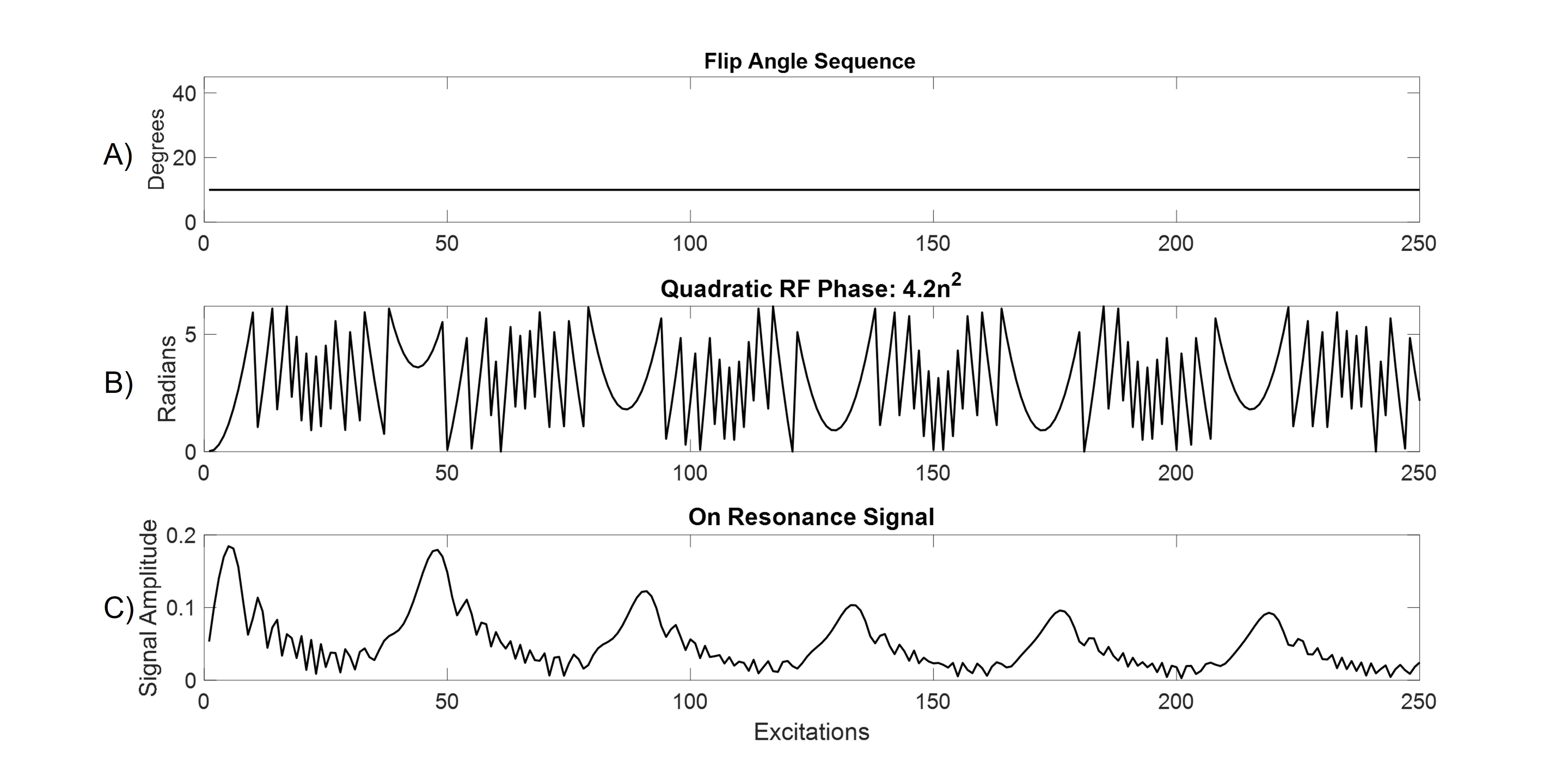
Pulse Sequence

A qRF-MRF sequence was implemented on a Philips Elition X 3 Tesla scanner (Philips Healthcare, Best, Netherlands) using a 32-channel receive coil array. The sequence’s flip angles and excitation RF phases are plotted in Figures 1a and 1b. It had balanced gradient areas and used a six-shot spiral readout with constant TR = 15.5 ms, TE = 2.2 ms, 10° flip angle, a spiral acquisition window of ~10 ms and acquired voxel size of 1.72 mm x 1.72 mm x 4 mm. A quadratic excitation pulse RF phase of 4.2n² degrees for n = 250 TRs sensitized the sequence to off-resonance. Figure 2 illustrates this: The quadratic phase corresponds to a repeating frequency sweep, and as the sequence sweeps past each resonance frequency, signals at that frequency are refocused and increase in amplitude for several TRs, before decaying again as the sequence’s frequency shifts away. Signals at different frequencies refocus at different time points, enabling an MRF dictionary match for off-resonance based on the signals’ amplitude and phase. A comparable conventional GRE-EPI (5 echoes per TR) sequence was also implemented, which used a 12 ms TE, 5 slices, 130 ms TR, 20° flip angle (the Ernst angle for this T₁ = 2000 ms phantom), and acquired voxel size of 0.43 mm x 0.54 mm x 5 mm. Both the qRF-MRF and GRE-EPI sequences imaged a 110x110 mm² FOV.

MRF Dictionary Construction

The qRF-MRF spiral data were gridded and coil-combined, and each voxel’s data were matched against entries of a Bloch-simulated dictionary. The dictionary was constructed for a single T₁ value (2000 ms), a range of 21 T₂ values from (10 to 200 ms), 4 initial M_z values (0.4, 0.5 0.6 1), and 1024 temperature values (-10 to 40 °C) across 250 excitations/timepoints.

Laser Heating Experiment

A phantom comprising 1% agar by volume of water was heated using a Class 3b BWTek BWF5-980-15 laser ablation system (Plainsboro, NJ) at 3W of continuous wave mode using a 400-micron optical fiber. Images were acquired as transverse slices perpendicular to the fiber. The dynamic scan time was 5.3 ms per image for GRE-EPI, and 3.9 ms per image for qRF-MRF. A 1 second relaxation delay was inserted between each 250-TR qRF-MRF block.

Intermittent Interfering Signal Simulation

To demonstrate qRF-MRF's robustness to intermittent interference from, e.g., the flow of water in transcranial MR-guided focused ultrasound, a simulation was performed in which signal from an unheated blinking circle was added to simulated qRF-MRF and 2DFT signals generated by a circular object with a centered Gaussian hot spot. The blinking circle’s amplitude was randomly varied through the scans up to 4x the main circle’s amplitude. qRF-MRF and 2DFT temperature maps were reconstructed for comparison.

Results and Discussion

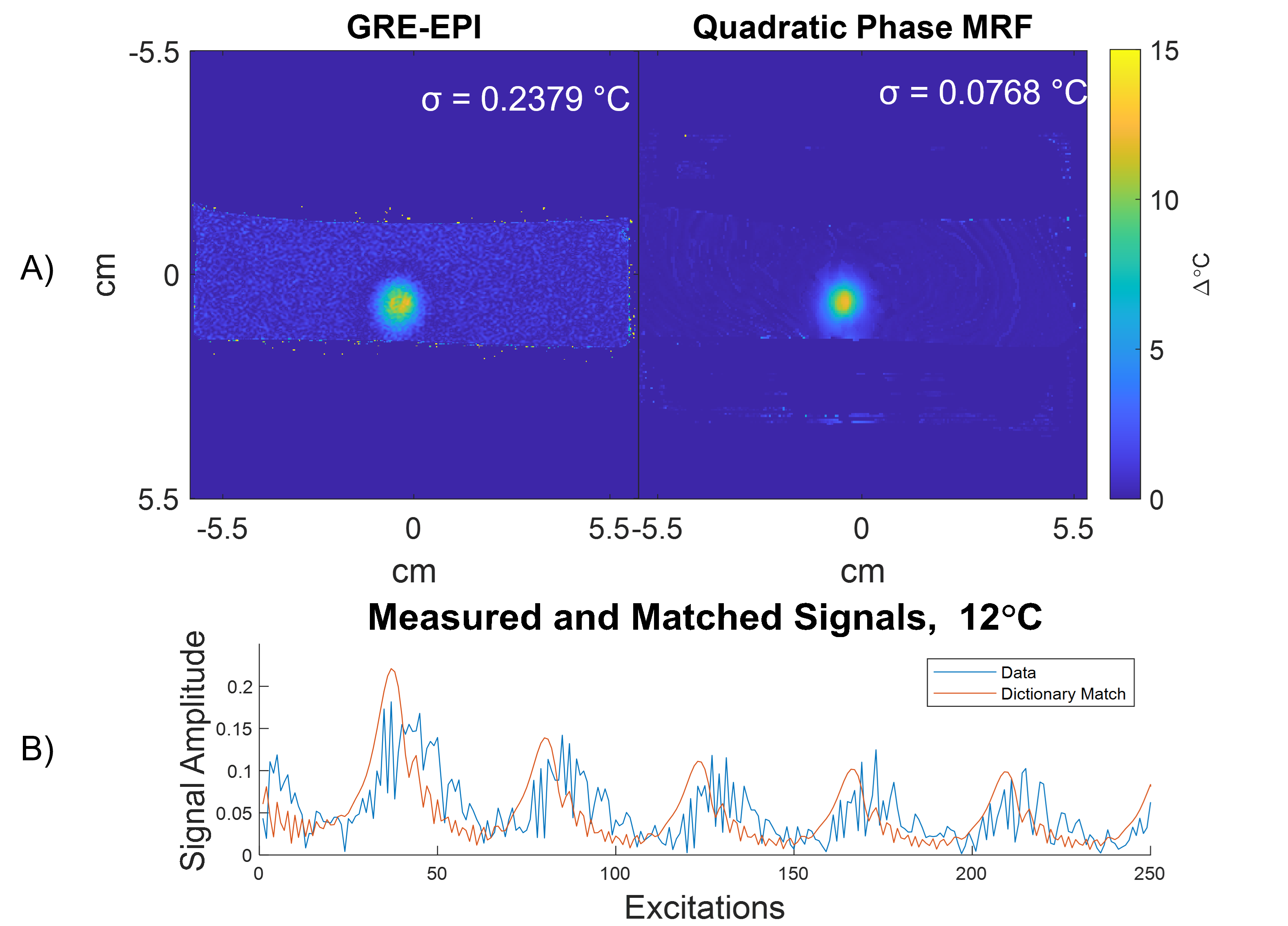
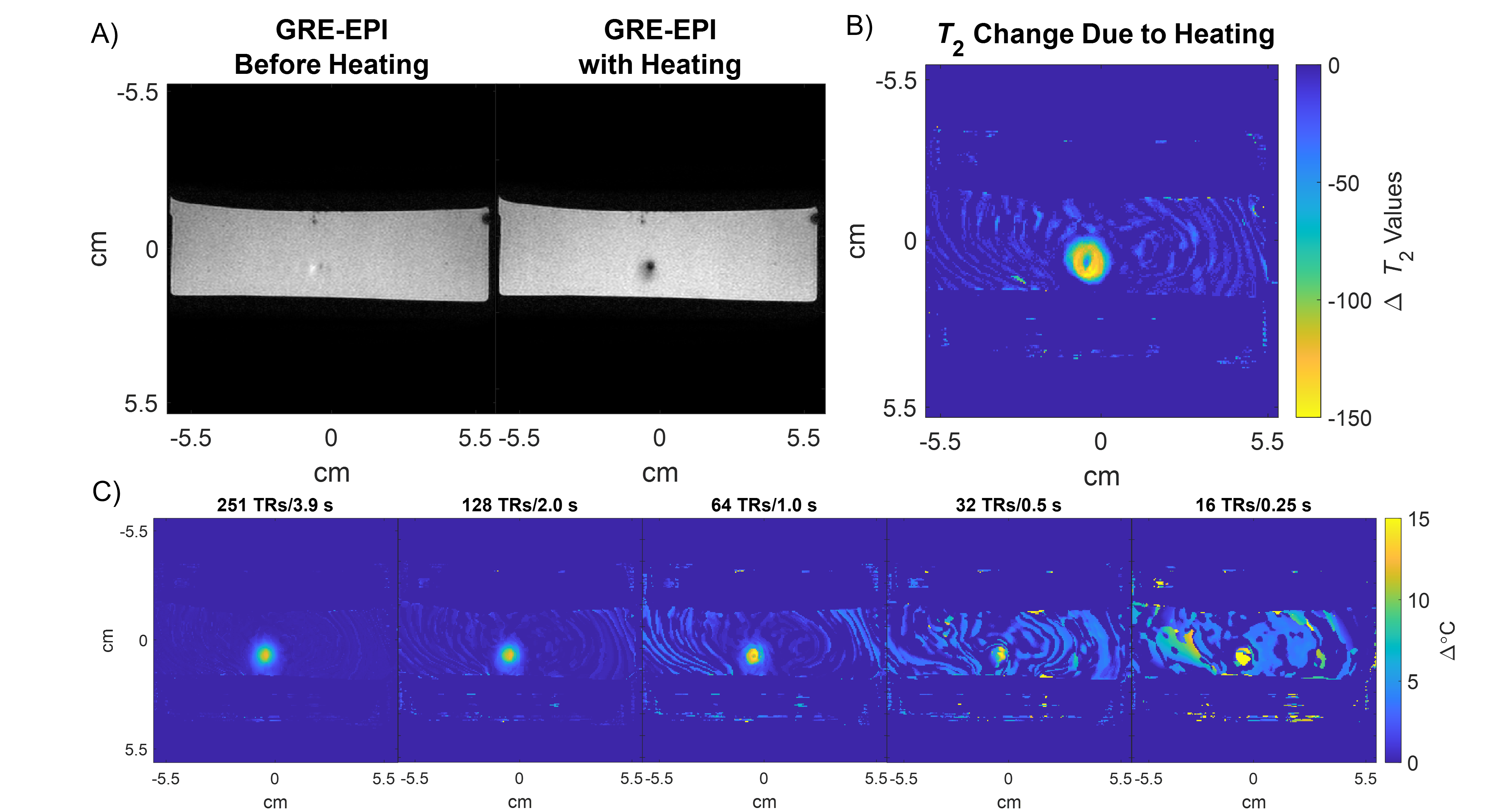
Figure 3a shows GRE-EPI and qRF-MRF temperature maps after the laser was switched off, as well as the matched and measured signal time courses for a heated voxel. The GRE-EPI temperature precision was ~3x worse than qRF-MRF's precision. Figure 4 shows how qRF-MRF can further produce a map of the change in T₂ caused by heating (4b), which corresponds to decreased signal amplitude in the GRE-EPI images (4a). Figure 4c shows that it may be possible to reduce the qRF-MRF block length by 2x or more without significant loss of temperature precision and accuracy. Figure 5a shows the centered circle object containing the hot spot, and Figures 5b shows the reconstructed 2DFT and qRF-MRF temperature maps. The qRF-MRF temperature error was > 3x lower than the 2DFT error (0.155 versus 0.487 °C RMS errors).

Conclusion

Results showed that qRF-MRF temperature mapping can provide precise temperature imaging while simultaneously generating maps of T₂ changes. The method’s short TE and repeated sampling of the center of k-space every TR retains signal as T₂ shortens with heating, unlike conventional PRFS scans which use long TEs for high temperature phase contrast and suffer loss of temperature precision with heating. The scan could be used with dynamic scan times as short as 2 seconds, and in a sliding window fashion, and is robust to intermittent interfering signals.

Acknowledgements

This work was supported by NIH grants R01 NS120518 and R01 EB028773.