Synopsis

Keywords: Image Reconstruction, Brain

Head motion can lead to artifacts in MR images. One source of motion artifacts is dynamic nonlinear variation in the background magnetic field (B₀). Fully accounting for this variation is computationally intractable. We proposed an efficient method of performing this correction by making use of principal component analysis and considering only a few dominant modes. We applied our method to measured data and compared the results to the case with no correction as well correction using a previous K-means based method.

Introduction

MRI is prone to motion-induced artifacts. One potential source for these artifacts is the fact that head motion can lead to spatially nonlinear dynamic changes in the background polarizing magnetic field (B₀) due to the static B₀ shim setting and motion-induced spatial changes of magnetic susceptibility in the head and torso¹. The resulting artifacts become much more pronounced at higher field strengths (e.g. 7T) and in methods focusing on the susceptibility effect such as T₂^*-weighted MRI. Therefore, in order to fully take advantage of high-field MRI’s unique ability to image fine scale structures, the effect of motion-induced nonlinear B₀ fluctuation must be corrected for. Several works have attempted to address this issue^2-4. Performing the correction on a shot-by-shot basis is computationally expensive. Here, we proposed an efficient method based on principal component analysis (PCA) of the B₀ effect on MRI signal⁵ and compared with another method using K-means clustering⁴.

Methods

Principle of PCA-based B0 correction
The forward equation for how MR signal is affected by the B₀ field (unit hertz) is:
$$s(k(t))=M\cdot\mathcal{FT}\{e^{2i\pi\,TE\,B_0(r,t)}\rho(r)\}.$$
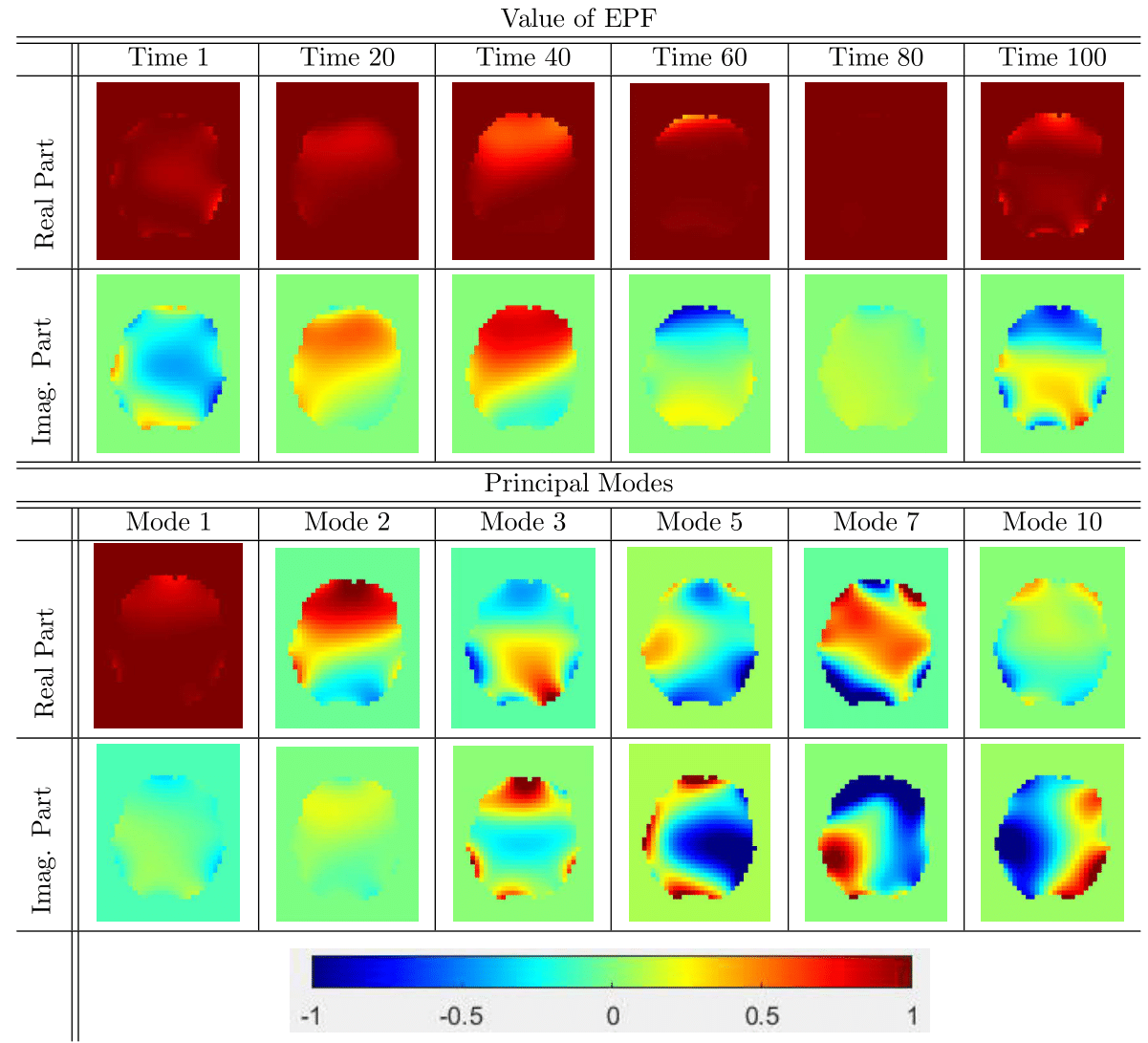
Here, $$$s$$$ is the signal, $$$\rho$$$ is the underlying image, $$$TE$$$ is the echo time, $$$\mathcal{FT}$$$ is the Fourier transform, and $$$M$$$ is the motion operator (for simplicity, B₁ sensitivity is omitted here). Directly solving this equation would require as many FTs as there are B₀ measurements, which is computationally intractable. To efficiently perform the correction, we approximated the exponential phase factor (EPF) from the equation above with a sum of a few principal components (as proposed by Wilm et. al⁵).
$$\text{EPF}=e^{2i\pi\,TE\,B_0(r,t)}\approx\sum_{j=1}^Lb_j(r)c_j(t).$$
Here, $$$b_j(r)$$$ is the jth principal mode or component, $$$c_j(t)$$$ is the weight of mode j at time t, and $$$L$$$ is the number of components that was used to perform the approximation.
Example values of the EPF and its corresponding principal modes are presented in Figure 1.
Plugging this decomposition into the forward equation, we obtained:
$$s(k(t))=M\cdot\sum_{j=1}^Lc_j(t)\mathcal{FT}\{b_j(r)\rho(r)\}.$$
The solution of the above equation now only requires L FTs.

MRI Experiment
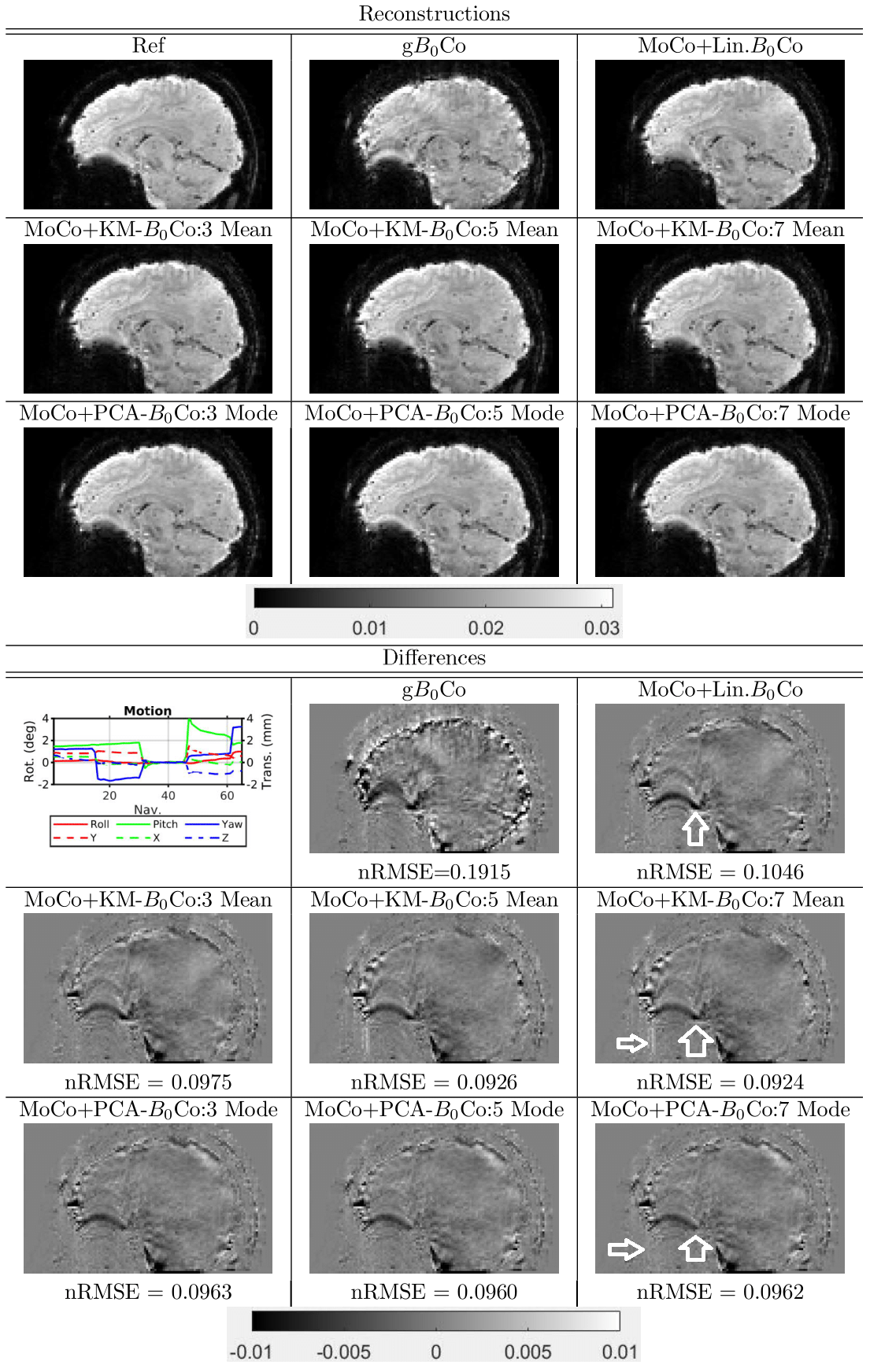
We performed two sets of experiments to evaluate the proposed correction algorithm. In Experiment I, eight healthy subjects (age:46±20, 4 males) were recruited and scanned on a 3T MRI (Prisma, Siemens). Subjects were instructed to stay relaxed, and the B₀ changes in the brain during eight-minute time windows were measured using a 3D EPI sequence (resolution:6x6x14mm³, FOV:240x180x144mm³, TE:4.2ms, and volume TR:0.65s). The scans were repeated 6 times for each subject. B₀ changes in the head frame were estimated from the co-registered EPI phase data. The obtained data was used to evaluate the validity of our approximation to the EPF. The data was also used to perform simulations where the corruption to a known image was simulated using the measured B₀ changes (TE:60ms) and the correction was applied to the corrupted image. In Experiment II, we considered 3D T₂^*-weighted MRI at 3T (isotropic 2mm resolution, TE:32ms, and FOV:240x180x120mm³). Two (male) subjects were recruited. Subjects were instructed to move their head, and a separate scan served as the reference when subjects stayed still. 3D EPI-based navigators were acquired with spatial resolution of 6x5.6x6mm³ and temporal resolution of 0.5s (for details see Liu et.al⁴). The T₂^*-weighted images were reconstructed with different corrections (see Figure 4). The reconstruction performance was evaluated based on the normalized root mean square error (nRMSE) against the reference scan.

Results

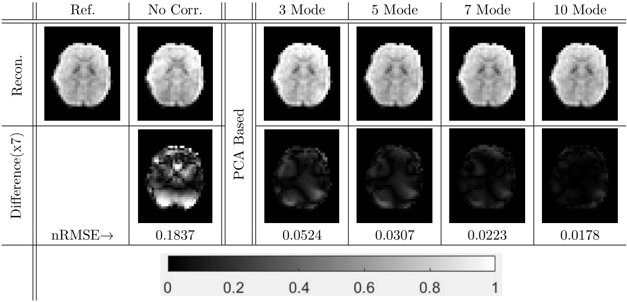
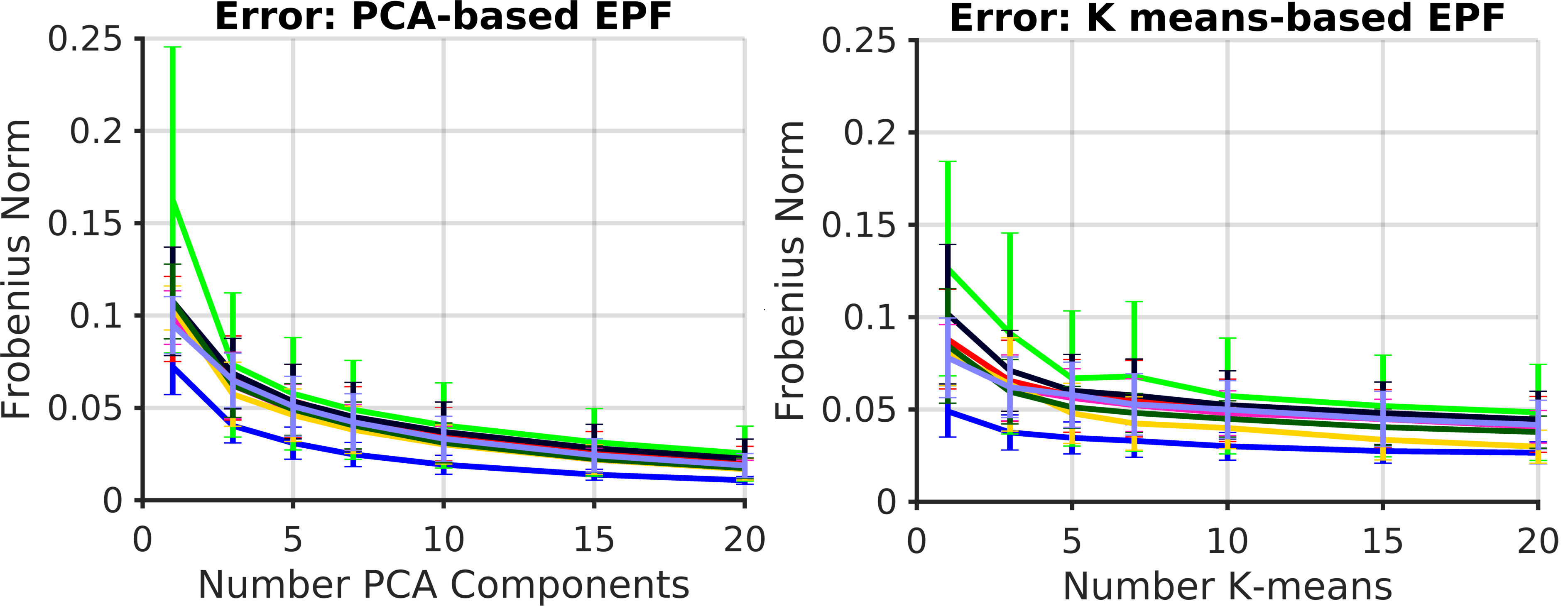
The results for an example simulation are presented in Figure 2. We observed that the reconstructions were improved by correcting for the nonlinear B₀ fluctuations. The correction improved with more PCA modes and reached a point after which including additional modes did not significantly improve the reconstruction.
We also directly evaluated the validity of our approximate EPF by computing the normalized Frobenius norm of the difference between the full and approximate EPFs. The results for this comparison for all subjects were summarized in Figure 3. The approximation was performed using both PCA and K-means. For a small number of modes/means, K-means slightly out-performed PCA, but as the number of modes/means increased, PCA performed better than K-means.
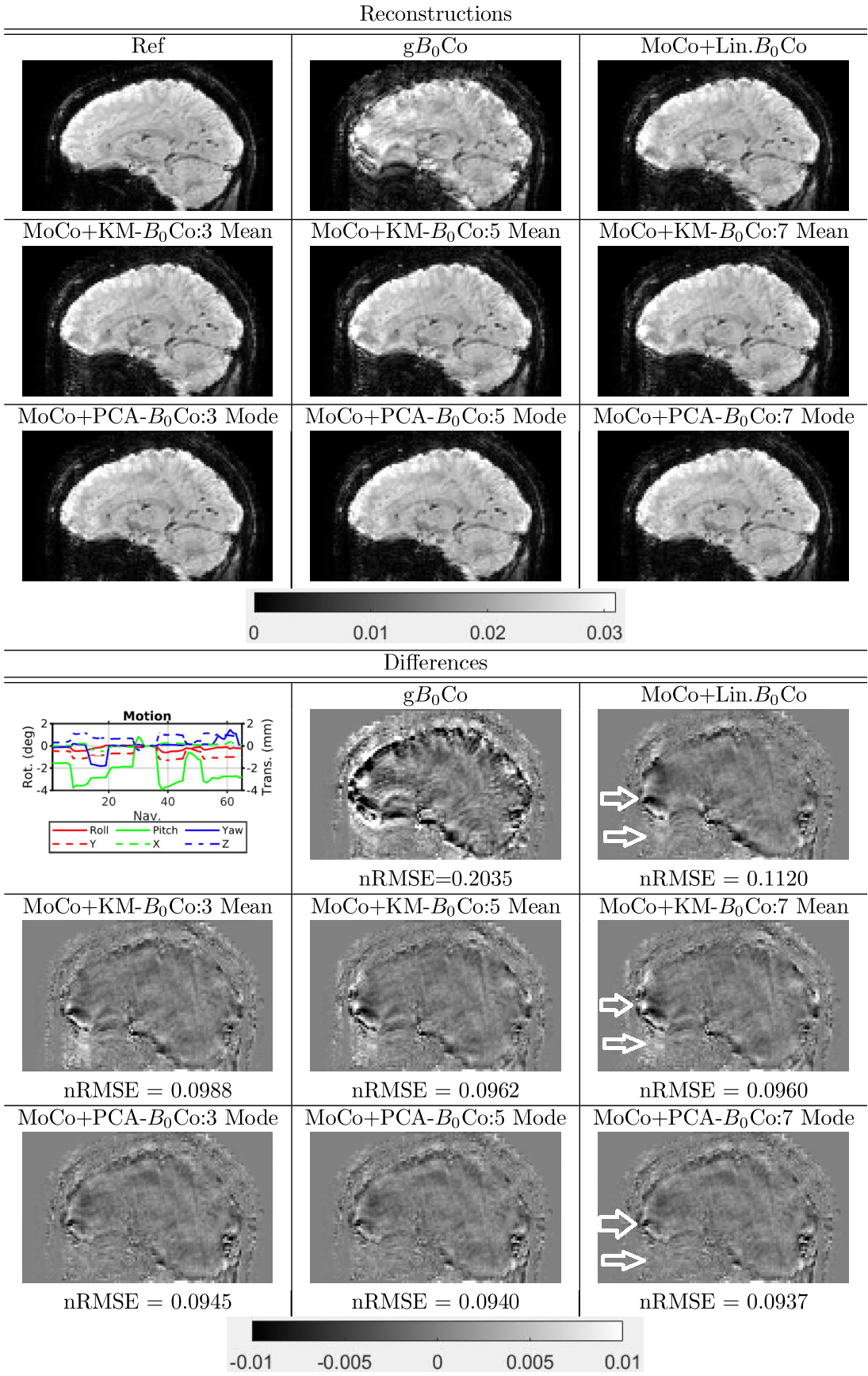
The results for experiments where subjects were asked to intentionally move, are presented in Figures 4 and 5. We observed that performing a nonlinear correction improved the reconstruction as compared to only a linear correction. The difference between PCA and K-means based reconstructions was not significant from an nRMSE perspective, but we did observe some qualitative improvements in PCA based reconstructions (denoted by arrows). We noted that motion (especially pitch) was greater for subject 1 than 2, we correspondingly observed more artifacts in subject 1. We observed that the overall reconstruction times for PCA and K-means based reconstructions were similar when the number of modes and means was the same.

Discussion and Conclusions

In this work, we showed that PCA can be used to efficiently correct for motion-induced nonlinear B₀ changes. PCA-based correction performed similarly to the previously established K-means based approach⁴ from an nRMSE perspective, with some qualitative improvements observed in PCA-based reconstructions. Systematic evaluation of this approach and other methods, such as the K-means approach, in a larger subject population is warranted in future studies to further establish its efficacy in high field and B₀-sensitive applications, such as T₂^*/susceptibility-weight MRI.

Acknowledgements

The authors gratefully acknowledge funding through the UT Southwestern faculty startup fund. We would also like to thank Yujia Huang for his help with data acquisition.