Synopsis

Keywords: Image Reconstruction, Artifacts, SPEN

The reconstruction theory of Spatio-temporal encoding MRI is not complete at present. Aliasing artifacts in SPEN MRI reconstructions can be traced to image contributions corresponding to high-frequency k-space signals. The k-space picture provides the spatial displacements, phase offsets and linear amplitude modulations associated to these artifacts, as well as routes to removing these from the reconstruction results. These new ways to estimate the artifact priors were applied to reduce SPEN reconstruction artifacts on simulated, phantom and human brain MRI data.

Introduction

Spatiotemporal encoded MRI (SPEN) has a unique advantage in reducing the distortion of fast imaging^1-4. Many super-resolved reconstruction methods based on the point spread function model provide stable reconstruction performance of under-sampled data, but all of them inevitably have a special class of boundary shift artifacts^5-8. The present study discusses an alternative description of SPEN MRI, based on a k-space data representation. Such k-space modeling can simplify the quantitative description of the experiment, and lead to descriptions of artifacts and their relation to subsampling, which are simple to grasp based on common criteria. The description also leads to a new way to estimate artifacts originating from sharp image transitions (“edges”), from which a novel image reconstruction method was proposed.

Methods

SPEN uses a unique linear sweep pulse to replace the excitation pulse or refocusing pulse in the conventional SE-EPI, which makes the encoding method superimpose a secondary phase factor along the phase encoding direction in the image domain. According to the time-frequency property of Fourier Transform, this coding property can be equally-described as the convolution of the conventional k-space with the Fourier form of the introduced quadratic phase, namely:
$$\rho_{\text {spen }}(y)=\rho(y) \cdot e^{-i C y^2} \stackrel{F T}{\Leftrightarrow} \tilde{\rho}_{\text {spen }}(f)=\tilde{\rho}(f) * \sqrt{\frac{\pi}{C}} e^{-i\left(\frac{\pi^2 f^2}{C}-\frac{\pi}{4}\right)}$$
The wavy line on the symbol represents the k-space data, and C is the coefficient of SPEN encoding feature, which is determined by the time-bandwidth product $$$Q=C \times F O V_y^2$$$. The frequency encoding direction is consistent with the conventional model, so it is not explicitly stated here. the quadratic phase leads to significant amplitude modulations of the signal in addition to the k frequency encoding, which need to be accounted for.
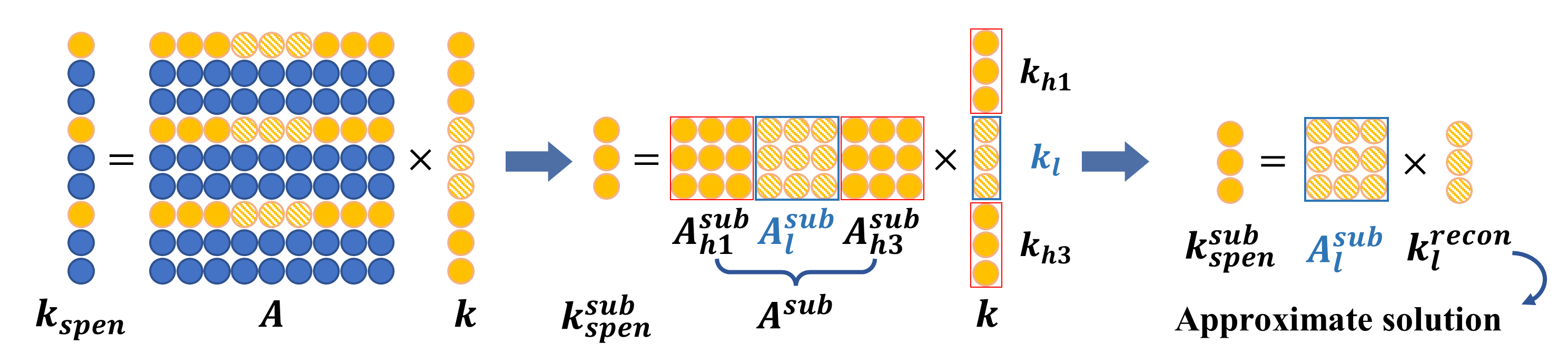
The undersampling results in the loss of the independent constraint of the coding system and the unsolvable inverse problem. For conventional medical images, their energy is often concentrated in low-frequency components, and the intensity of the central region of k-space is much stronger than that of other locations. Directly setting the k-space data of the non-central region in the direction of phase coding zero until the amount of existing data is sufficient to support the solution of the reconstructed inverse problem. In this approximation method, the high-frequency component is discarded and compressed into the low-frequency component by undersampling, so that the large-interval wide-band SPEN data can be converted into the small-interval narrow-band conventional MRI data. The distortion of the reconstruction result can be described as:
$$k_l^{\text {recon }}=\left(A_l^{\text {sub }}\right)^{-1} \cdot A^{\text {sub }} \cdot k^{\text {true }}=k_l^{\text {true }}+\sum_{s=1}^{R-1}\left(A_l^{\text {sub }}\right)^{-1} \cdot A_{h(s)}^{\text {sub }} \cdot k_{h(s)}^{\text {true }}$$
Where 'l' and 'h' respectively describe the low-frequency and high-frequency components of the response object, ‘A’ refers to the matrix of SPEN encoding, 'sub' refers to the subspace after under-sampling, and the second term describes the accumulation of high-frequency signal features at different positions. The features of the transformation matrix of high-frequency data are quantified, and the coding properties matching the features of the image domain are obtained. The details are shown in FIG 1.
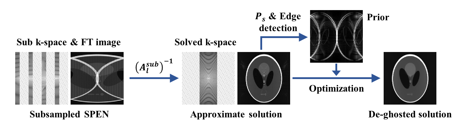
We obtain a weighted factor of image space with proper estimation, which is combined with the TV constraint of L1 regularization to form an optimization objective with the data fidelity term. This process effectively attenuates artifacts, as FIG 2 shows.

Results and Discussion

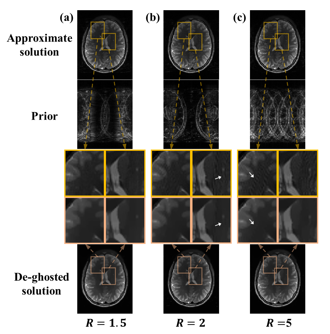
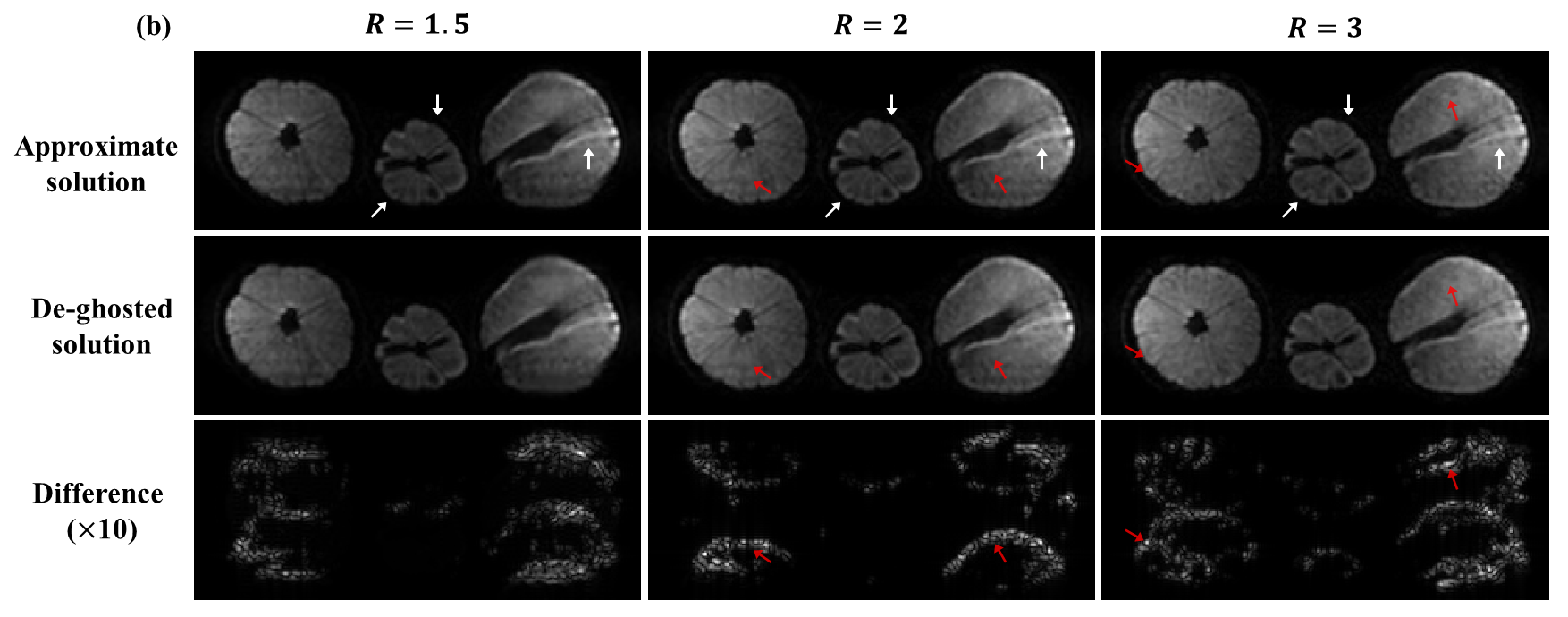
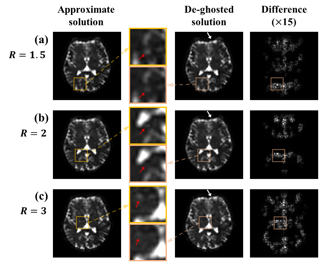
FIG. 3 records the results under simulation data. Under various undersampling modes, the artifacts in the approximate solutions have different representations, but all of them are roughly similar to the artifact estimation priors and can be effectively removed in further optimization. FIG. 4 shows the results of 2 oranges and 1 lemon’s imaging. These fruits have cavities at their center and effects at their surfaces, which can lead to marked field inhomogeneity-driven distortions (white arrows). The distortion effect is decreased as the undersampling rate increase. The difference between the approximate solution and the optimized image has a similar distribution to the estimated artifacts. FIG. 5 records the brain with acquisition data. Again, the error performs a great similarity to the estimated ghost, and the removal or weakening of the undesired feature can be seen in the zoom-in diagram.

Conclusions

A k-space description of SPEN’s reconstruction helps to better understand the signal characteristics of this MRI technique, and to improve the quality of its resulting images

Acknowledgements

This work is supported by the National Natural Science Foundation of China (No. 62001290), Shanghai Science and Technology Development Funds (21DZ1100300), sponsored by the National Science and Technology Innovation 2030 Major Project (2022ZD0208601), and by the Israel Science Foundation (grants 3594/21 and 1874/22).