Synopsis

Keywords: Electromagnetic Tissue Properties, Electromagnetic Tissue Properties

Our results suggest that R2* maps in UK Biobank are confounded by the macroscopic field variation which leads to spurious associations driven by field variations due to the air/tissue interfaces. This effect can be modeled as a signal modulation which can be removed through a voxel-wise correction.

Introduction

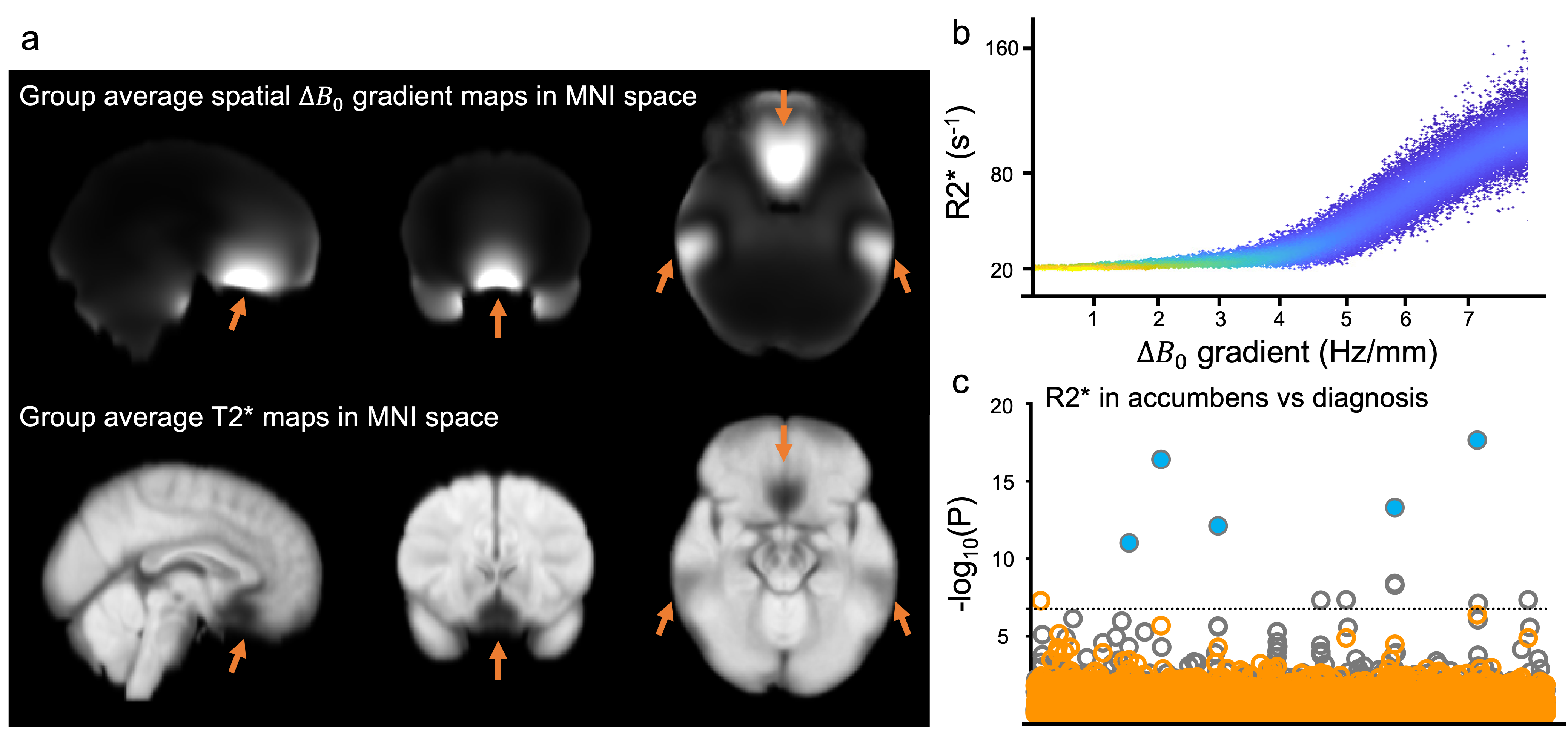
Mapping of the R2* (1/T2*) relaxation rate has multiple important applications in MRI, including quantitative assessment of susceptibility-shifted sources such as iron and myelin content in brain tissue¹. R2* maps can be obtained from a multi-echo gradient echo (mGRE) acquisition through a simple exponential fitting of the signal decay profile. However, estimation of a biologically-meaningful R2* is prone to errors, as multiple confounding factors can additionally contribute to the signal decay. One such confound is macroscopic $$$B_{0}$$$ field variations across a voxel (Δ$$$B_{0}$$$), where the presence of spatial Δ$$$B_{0}$$$ gradients lead to additional dephasing and faster signal decay². This results in an overestimation of R2*, particularly in data acquired with a large voxel size³.

Despite the advantages of high spatial resolution, there are situations where large voxel dimensions are preferable. In UK Biobank (UKB), thick slices enable the acquisition of mGRE data in 2.5mins in 100,000 subjects. However, confounding effects of Δ$$$B_{0}$$$ gradients might lead to spurious associations. For example, geometry of the sinuses could lead to apparent T2* differences that are unrelated to microscopic features like tissue iron or myelin⁴. Fig. 1a shows a group-average (slice-direction) spatial Δ$$$B_{0}$$$ gradient map and corresponding group-average T2* map in UKB. Regions with high Δ$$$B_{0}$$$ gradients exhibit high R2*, including near the sinuses (Fig 1b). High Δ$$$B_{0}$$$ gradients in some deep gray regions like the accumbens may be responsible for apparent associations between R2* and diagnosis of nasal polyps observed in UKB⁴.

The aim of this work is to implement a physics-informed correction method³ to enable accurate voxel-wise estimation of R2* in UKB that accounts for variations in spatial Δ$$$B_{0}$$$ gradients. Using simulations and phantom scans, we demonstrate that the proposed physical model can explain the confounding effect of Δ$$$B_{0}$$$ gradients on R2* estimates.

Methods

Signal modulation model

For the UK Biobank GRE protocol, as the in-plane resolution is much higher than the slice thickness, we only consider spatial Δ$$$B_{0}$$$ gradients along the z-direction. The GRE signal can be modelled as³: $$S(TE,z_{0})=e^{-R_2^*TE}e^{j2\pi\gamma{ΔB_{0}(z_{0})}TE}\times\int_{R}S_{0}e^{j2\pi\gamma[{ΔB_{0}(z)-{ΔB_{0}(z_{0})}]}TE}\cdot{SRF(z-z_{0})}dz$$ where $$$S(TE,z_{0})$$$ is the measured signal at $$$TE$$$ and location $$$z_{0}$$$, $$${\gamma}ΔB_{0}(z)$$$ is the magnetic field offset (in Hz), and $$$SRF(z-{z}_0)$$$ is the spatial response function (SRF) of a voxel centered at $$$z_{0}$$$. This model indicates that in the presence of spatial Δ$$$B_{0}$$$ gradients, the signal is additionally modulated by the term $$$\int_{R}S_{0}e^{j2\pi\gamma[{ΔB_{0}(z)-{ΔB_{0}(z_{0})}]}TE}\cdot{SRF(z-z_{0})}dz$$$, which will decay faster for larger Δ$$$B_{0}$$$ gradients or thicker slices. Removal of this modulation term from the magnitude images before R2* estimation enables correction for the effect of Δ$$$B_{0}$$$ gradients.

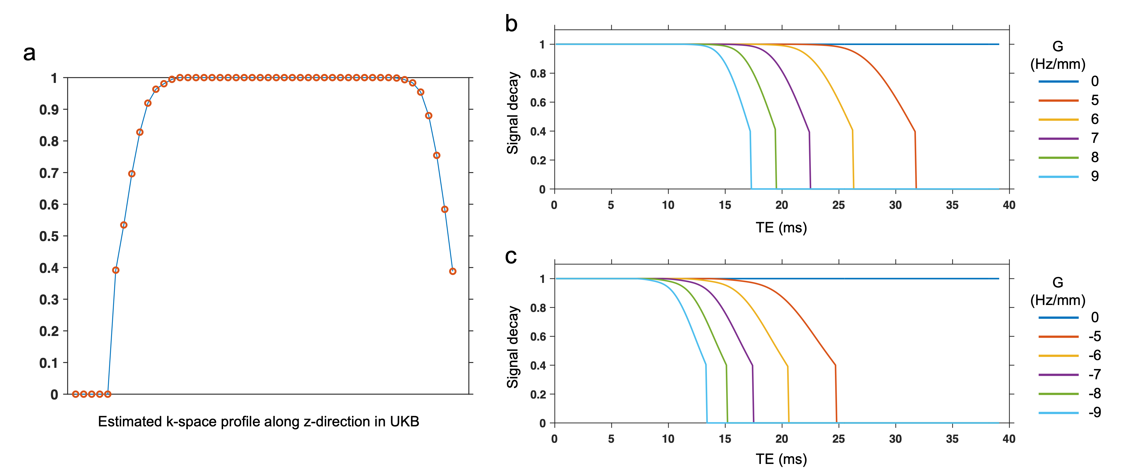
SRF is the Fourier transformation of the k-space profile in UKB protocol, which can be estimated by simulating the image reconstruction chain (including image filters) with a digital phantom using the Siemens ICE simulator. Spatial Δ$$$B_{0}$$$ gradient maps were estimated by taking the gradient magnitude of the macroscopic field Δ$$$B_{macro}$$$ map, which was calculated as: $${\gamma}B_{macro}={\gamma}B_{average}-{\gamma}B_{vsharp}$$ where $$${\gamma}B_{average}$$$ is two-echo averaged and unwrapped (using PRELUDE⁵) filed map. $$${\gamma}B_{vsharp}$$$ is V-SHARP⁶ filtered $$${\gamma}B_{average}$$$.

Phantom data acquisition

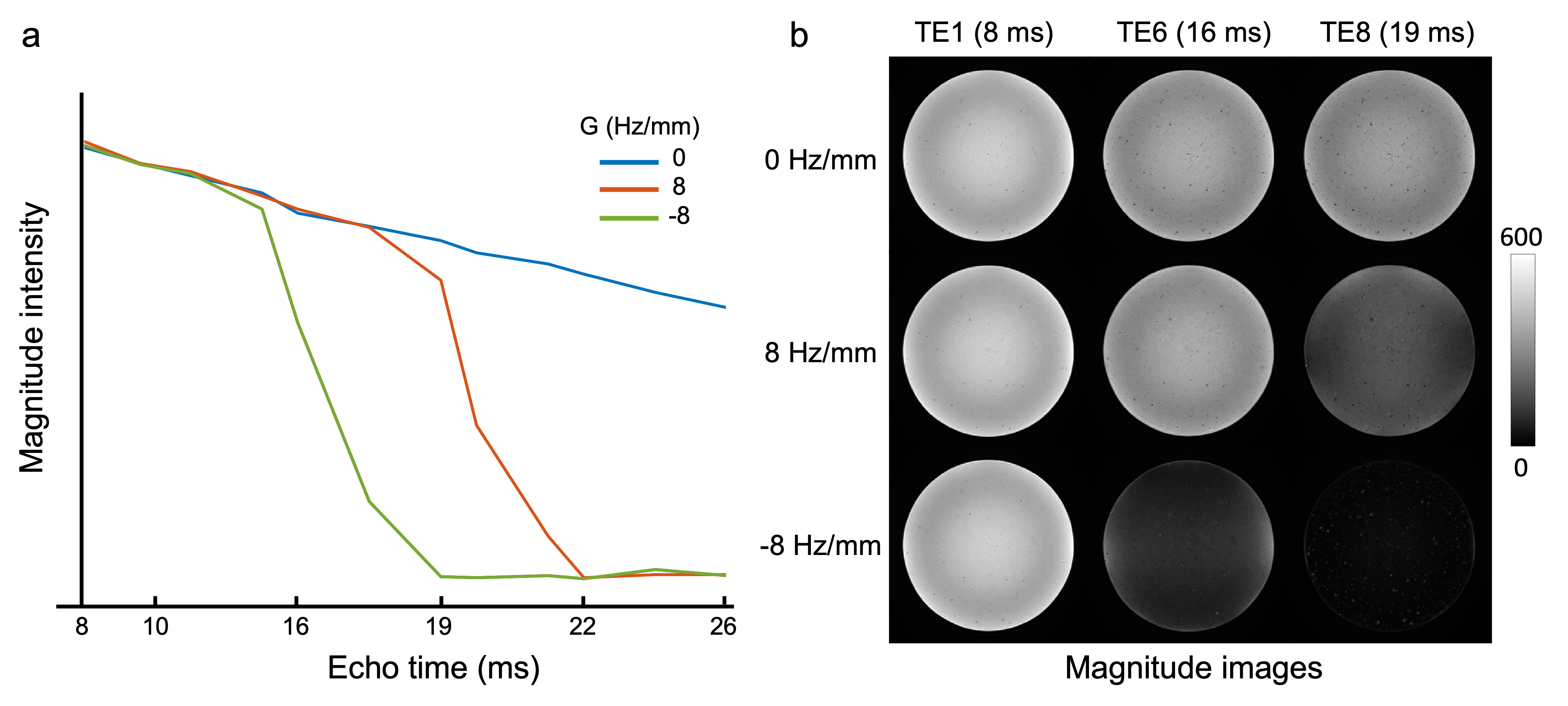
To establish the link between estimated SRF, spatial gradients and signal modulation, we further acquired phantom data using the UK Biobank protocol: 3D dual-echo GRE, TE1/TE2/TR=9.4/20/27 ms, 0.8x0.8x3 mm, matrix 256x288x48. We acquired 14 repeats with a varying linear field gradient (0-9.5 Hz/mm) along the slice-direction. To investigate the signal evolution of the GRE data, we additionally acquired three 12-echo acquisitions (TEs=8-26 ms) with a linear field gradient of -8, 0 and 8 Hz/mm respectively.

Results

The SRF of UK Biobank GRE data was calculated as the Fourier transformation of the estimated k-space profile (Fig. 2a). We simulated the signal modulation in the presence of a linear Δ$$$B_{0}$$$ gradient, noted as $$$G$$$. The use of slice-direction partial Fourier in UKB results in an asymmetric k-space profile (Fig. 2a), making the signal modulation dependent on the direction of the gradient (Fig.2b, c).

For experimental data, the link between the direction of $$$G$$$ and signal decay profile must be estimated before applying any correction. Here we used the 12-echo phantom data to analyze this link (Fig. 3). As expected, the presence of spatial Δ$$$B_{0}$$$ gradients led to faster signal decay, with the different decay profiles for positive/negative $$$G$$$ being consistent with the simulations in Fig. 2.

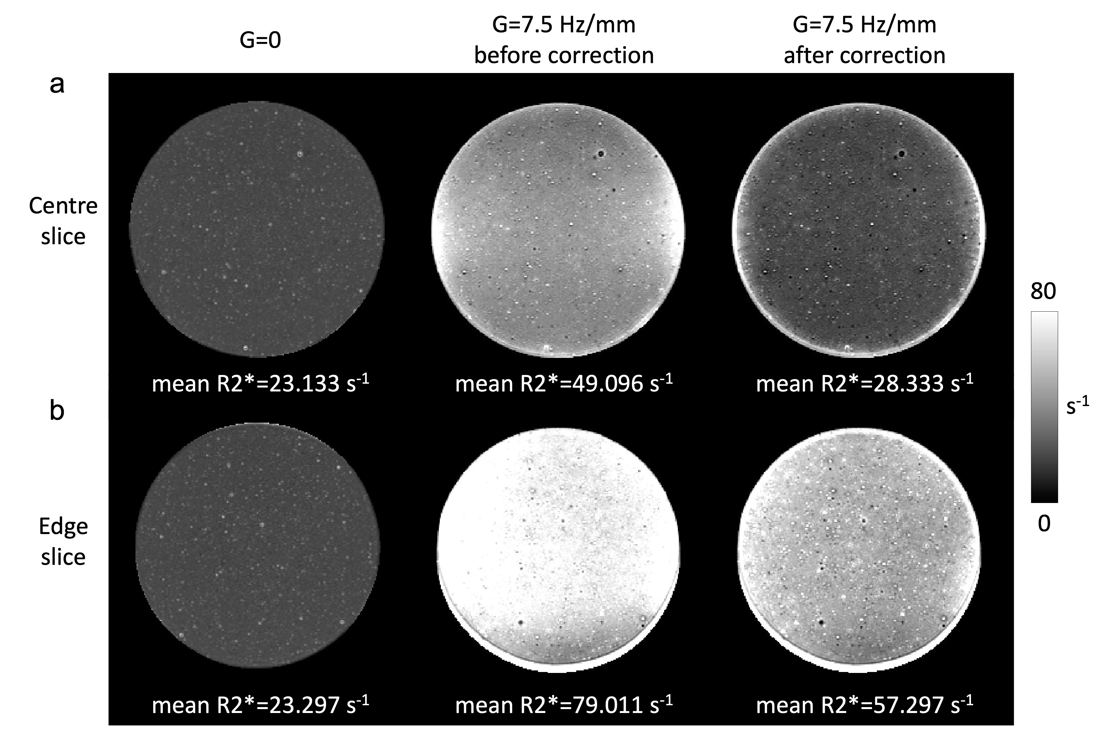
Combining the signal modulation model and signal decay profile, we performed a voxel-wise correction for the dual-echo phantom data. Figure 4 shows the comparison of example R2* maps generated before and after correction, in the presence of a linear 7.5 Hz/mm field gradient. The proposed method was able to restore R2* values in voxels located in the centre of the phantom (Fig. 4a), but voxels near the edge of the phantom showed remaining overestimation of R2* (Fig. 4b).

Discussion

Our results suggest in vivo R2* maps in UKB are confounded by the presence of spatial Δ$$$B_{0}$$$ gradients, which can be modeled as a signal modulation relating to the value of the Δ$$$B_{0}$$$ gradient in each voxel and echo times. Ιn UKB, our empirical results suggest this is predominately driven by air/tissue interfaces. Future works include accounting for the change of modulation in voxels near the edge of the field-of-view, validation using newly acquired in vivo datasets, and implementation in UKB.

Acknowledgements

Karla L. Miller and Benjamin C. Tendler contributed equally to this work.