Synopsis

Keywords: Image Reconstruction, Image Reconstruction

Radial sampling is a fast magnetic resonance imaging technique. The projected fast iterative soft-thresholding algorithm (pFISTA) has shown the advantage to solved tight frame sparse reconstruction model for removing undersampling image artifacts. However, the convergence of this algorithm under radial sampling has not been clearly set up. In this work, the authors derived a theoretical convergence condition for this algorithm and an optimal step size was further suggested to allow the fastest convergence. Verifications were made in vivo data of static brain imaging and dynamic contrast-enhanced (DCE) liver imaging, demonstrating that the recommended parameter allowed fast convergence in radial MRI.

Purpose

Magnetic resonance imaging (MRI) is a non-invasive and non-radioactive imaging technique that has been widely used in medical diagnosis. However, one of its limitations is long time cost. A projected fast iterative soft-thresholding algorithm (pFISTA) was proposed to achieve fast and low-error reconstruction [1]. its advantage is less requirement on memory space and a simpler algorithm setting [1-3]. Radial sampling MRI shows robustness to object motion [4-7] , e.g. vigorous patient activities in brain imaging [8], movement of liver or heart in free-breathing dynamic imaging [9-11]. With more practices of radial sampling, however, we found that it is hard to make pFISTA converge on different datasets. A comprehensive convergence analysis of pFISTA under radial sampling is lacking.

Method

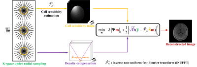
For static radial MRI reconstruction (Fig. 1), the target image $$$\mathbf{m}$$$ is reconstructed by solving the l1-norm minimization problem under a tight frame $$$\mathbf{\Psi}$$$ according to [1-3]: $$\mathop {\min }\limits_\mathbf{m} {\rm{ }}\lambda {\left\| {{\rm{\mathbf{\Psi}\mathbf{m}}}} \right\|_1} + \frac{1}{2}\left\| {\sqrt {{\rm{\mathbf{\tilde D}}}} ({\rm{\mathbf{\tilde y}}} - {\mathbf{\tilde {\cal F}}_{\cal N}}{\rm{\mathbf{\tilde S}\mathbf{m}}})} \right\|_2^2, \tag{1}$$where $$${\rm{\mathbf{\tilde y} = }}\left[ {{{\rm\mathbf{y}}_1}{;}{{\rm\mathbf{y}}_2}{;} \ldots {;}{{\rm\mathbf{y}}_J}} \right] \in \mathbb{C}{^{MJ}}$$$,$$${\rm{\mathbf{\tilde S} = }}\left[ {{{\rm\mathbf{S}}_1}{;}{{\rm\mathbf{S}}_2}{;} \ldots {;}{{\rm\mathbf{S}}_J}} \right]$$$,$$${\rm{{\tilde {\cal F}_{\cal N}} = }}\left[ {{{\rm{\cal F}}_{\cal N}}{;}{{\rm\mathbf{\cal F}}_{\cal N}}{;} \ldots {;}{{\rm{\cal F}}_{\cal N}}} \right]$$$,that saves k-space data, CSM and NUFFT operators of multi-coils, respectively. The $$${\left\| \cdot \right\|_1}$$$ and $$$ {\left\| \cdot \right\|_2}$$$ are the l₁ and l₂ norms, respectively. The is a regularization parameter that balances the sparsity and data consistency. The $$$ \lambda $$$ is a regularization parameter that balances the sparsity and data consistency.$$$\sqrt {\mathbf{\tilde D}} \in \mathbb{R}{^{MJ \times MJ}}$$$ represent density compensation.The reconstruction mosdel in Eq. (1) is solved with the pFISTA algorithm in an iterative manner:$${\mathbf{m}^{(k + 1)}} = {\mathbf{\Psi} ^*}{S_{\lambda \beta }}(\mathbf{\Psi} ({\mathbf{\hat m}^{(k)}} + \beta {\mathbf{\tilde S}^H}\tilde {\cal F}_{\cal N}^ * \mathbf{\tilde D}(\mathbf{y} - \tilde {\cal F}_{\cal N}^{}\mathbf{\tilde S}{\mathbf{\hat m}^{(k)}}))),\tag{2}$$where $$$k$$$ denotes the $$${k^{{\rm{th}}}}$$$ iteration,$$${\mathbf{\Psi} ^*}$$$ is the inverse transform of the tight frame $$${\mathbf{\Psi} }$$$,$$${\mathbf{\tilde S}^H}$$$ is the Hermitian transpose of $$${\mathbf{\tilde S}}$$$, $$$\tilde {\cal F}_{\cal N}^ * $$$ is the adjoint operator of the NUFFT operator $$$\tilde {\cal F}_{\cal N}$$$,$$${S_{\lambda \beta }}( \cdot )$$$ is an element-wise soft-thresholding operator defined as $$${S_{\lambda \beta }}(\alpha ) = \max \left\{ {\left| \alpha \right| - \lambda \beta ,0} \right\}\frac{\alpha } {{\left| \alpha \right|}}$$$ with the threshold $$$\lambda \beta$$$.The convergence of pFISTA highly depends on $$$\mathbf{B}$$$ under radial sampling, which is defined as$$\mathbf{B} = {\mathbf{\tilde S}^H}\tilde {\cal F}_{\cal N}^ * \mathbf{\tilde D}\tilde {\cal F}_{\cal N}^{}\mathbf{\tilde S}\tag{3}$$We were derived a theoretical convergence condition for this algorithm, the step size $$$\beta$$$ lies in the following range:$$0 < \beta \le \frac{1}{{{\mathbf{\sigma} _{\max }}(\mathbf{B})}} = \gamma\tag{4}
$$where $$${\mathbf{\sigma} _{\max }}(\mathbf{B})$$$ denotes largest eigenvalue of the $$$\mathbf{B}$$$ ,it is empirically estimated by using the power iteration [12], we define $$$\gamma = 1/{\mathbf{\sigma} _{\max }}(\mathbf{B})$$$ for simple notation.
For DCE MRI reconstruction (Fig. 2), all image frames are reconstructed by solving the following optimization problem:$$\mathop {\min }\limits_\mathbf{m} {\rm{ }}\lambda {\left\| {{\bf{Am}}} \right\|_1} + \frac{1}{2}\left\| {\sqrt {{\bf{\mathord{\buildrel{\lower3pt\hbox{$\scriptscriptstyle\frown$}} \over D} }}} ({\bf{\mathord{\buildrel{\lower3pt\hbox{$\scriptscriptstyle\frown$}} \over y} }} - {{\mathord{\buildrel{\lower3pt\hbox{$\scriptscriptstyle\frown$}} \over {\cal F}} }_{{\cal N}}}{\bf{\mathord{\buildrel{\lower3pt\hbox{$\scriptscriptstyle\frown$}} \over S} m}})} \right\|_2^2,\tag{5}
$$where $$${\rm{\mathbf{m} = }}\left[ {{{\rm\mathbf{m}}_1}{;}{{\rm\mathbf{m}}_2}{;} \ldots {;}{{\rm\mathbf{m}}_F}} \right] \in \mathbb{C}{^{NF}}$$$ is a long column vector, $$${\rm\mathbf{\mathord{\buildrel{\lower3pt\hbox{$\scriptscriptstyle\frown$}} \over y}= }}\left[ {{{{\rm\mathbf{\tilde y}}}_1}{;}{{{\rm\mathbf{\tilde y}}}_2}{;} \ldots {{{\rm\mathbf{\tilde y}}}_f} \ldots{;}{{{\rm\mathbf{\tilde y}}}_F}} \right] \in\mathbb{C} {^{JMF}}$$$ ,$$${\rm\mathbf{\mathord{\buildrel{\lower3pt\hbox{$\scriptscriptstyle\frown$}} \over S}= }}\left[ {{{{\rm\mathbf{\tilde S}}}_1}{;}{{{\rm\mathbf{\tilde S}}}_2}{;} \ldots {{{\rm\mathbf{\tilde S}}}_f} \ldots{;}{{{\rm\mathbf{\tilde S}}}_F}} \right] \in\mathbb{C} {^{JMF\times NF}}$$$ and $$${\mathord{\buildrel{\lower3pt\hbox{$\scriptscriptstyle\frown$}} \over {\cal F}} _{\cal N}}{\rm{ = }}\left[ {{{\tilde {\cal F}}_{\cal N}}{;}{{\tilde {\cal F}}_{\cal N}}{;} \ldots{;}{{\tilde {\cal F}}_{\cal N}}} \right] \in\mathbb{C} {^{JMF \times JNF}}$$$ saves the k-space data, sensitivity maps and NUFFT operators for multi-coils, respectively. The $$$\bf {\bf{A}}{\rm{ = }}\mathord{\buildrel{\lower3pt\hbox{$\scriptscriptstyle\frown$}} \over \Psi } {\cal P}$$$ represent the sparse transform operator.
Eq. (5) is solved by iteratively addressing the following sub-problems:
$$\bf {m^{(k + 1)}} = {{\cal P}^ * }{\mathord{\buildrel{\lower3pt\hbox{$\scriptscriptstyle\frown$}} \over \Psi } ^*}{S_{\lambda \beta }}(\mathord{\buildrel{\lower3pt\hbox{$\scriptscriptstyle\frown$}} \over \Psi } {\cal P}({\hat m^{(k)}}_{} + \beta {\mathord{\buildrel{\lower3pt\hbox{$\scriptscriptstyle\frown$}} \over S} ^H}\mathord{\buildrel{\lower3pt\hbox{$\scriptscriptstyle\frown$}} \over {\cal F}} _{\cal N}^ * \mathord{\buildrel{\lower3pt\hbox{$\scriptscriptstyle\frown$}} \over D} (\mathord{\buildrel{\lower3pt\hbox{$\scriptscriptstyle\frown$}} \over y} - \mathord{\buildrel{\lower3pt\hbox{$\scriptscriptstyle\frown$}} \over {\cal F}} _{\cal N}^{}\mathord{\buildrel{\lower3pt\hbox{$\scriptscriptstyle\frown$}} \over S} {\hat m^{(k)}}_{}{\rm{ }}))),\tag{6}$$where $$$\bf {\mathord{\buildrel{\lower3pt\hbox{$\scriptscriptstyle\frown$}} \over \Psi } ^*}$$$ s the adjoint operator of $$$\bf\mathord{\buildrel{\lower3pt\hbox{$\scriptscriptstyle\frown$}} \over \Psi }$$$, $$$ {\cal P}$$$ is an operator that extracts pixel values along the temporal dimension at a given spatial location.

Results

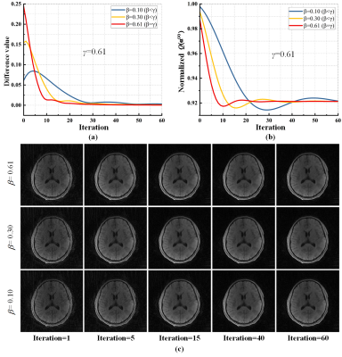
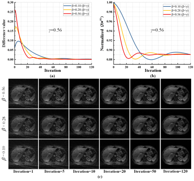
Results Brain data of 3 subjects and liver DCE data of 3 subjects are used in our experiments. Quantification criterion of empirical convergence includes, objective function value $$$Q({{\bf{\alpha }}^{(k)}})$$$ and the difference value between two successively intermediate reconstruction $$${{\bf{m}}^{(k + 1)}}$$$ and $$${{\bf{m}}^{(k)}}$$$. For static radial imaging, the difference value and objective function value were tested on the brain imaging data (Fig. 3), both difference value and objective function converged when $$$\beta \le \gamma$$$ and converged fastest when $$$\beta = \gamma$$$ . For the liver DCE imaging, $$$\beta \le \gamma$$$ ensures the convergence and $$$\beta = \gamma$$$ leads to the fastest convergence (Fig. 4).

Conclusion

In this work, under the radial sampling of static and dynamic MRI, we a derive theoretical convergence condition for the pFISTA in the tight-frame-based sparse image reconstruction and an optimal step size was suggested to ensure the fastest convergence. Experiments on in vivo data demonstrated that the recommended parameter allowed fast convergence in both static and dynamic radial sampling of MRI.

Acknowledgements

Funding: This work was financially supported by the National Key R&D Program of China (2017YFC0108703), National Natural Science Foundation of China (62122064, 61971361 and 52275575), Natural Science Foundation of Fujian Province (2020H6003), President Fund of Xiamen University (0621ZK1035) and Xiamen University Nanqiang Outstanding Talents Program. The corresponding authors are Gaofeng Zheng and Xiaobo Qu (Email: zheng_gf@xmu.edu.cn, quxiaobo@xmu.edu.cn).