4777
Analysis of Deep Learning-based Reconstruction Models for Highly Accelerated MR Cholangiopancreatography: to Fine-tune or not to Fine-tune
Jinho Kim1,2, Thomas Benkert2, Bruno Riemenschneider1, Marcel Dominik Nickel2, and Florian Knoll1
1Artificial Intelligence in Biomedical Engineering, Friedrich-Alexander-Universität Erlangen-Nürnberg, Erlangen, Germany, 2MR Application Pre-development, Siemens Healthcare GmbH, Erlangen, Germany
1Artificial Intelligence in Biomedical Engineering, Friedrich-Alexander-Universität Erlangen-Nürnberg, Erlangen, Germany, 2MR Application Pre-development, Siemens Healthcare GmbH, Erlangen, Germany
Synopsis
Keywords: Machine Learning/Artificial Intelligence, Image Reconstruction, Magnetic Resonance Cholangiopancreatography
MR cholangiopancreatography (MRCP) is a special MRI technique to visualize the biliary systems. Deep Learning-based (DL) reconstruction models have shown to reduce scan time from many anatomical regions. However, they generally require large training datasets. This is challenging for applications like MRCP, where public datasets are not available. This work analyzes two approaches to training a DL model for highly accelerated MRCP reconstruction: training from scratch using a small MRCP dataset and fine-tuning a model pretrained on a public knee dataset. Results show that despite of the substantial data domain shift between training and testing, fine-tuning outperformed training from scratch.Introduction
MRCP is an MRI technique that visualizes the biliary systems using a heavily T2-weighted sequence. Acquiring MRCP is challenging due to irregular breathing, causing undiagnostic images. Therefore, reducing scan times is very important for the MRCP exam, and techniques like parallel imaging1-2 (PI) and compressed sensing3 (CS) have already been employed successfully for MRCP4. DL methods have shown promising results in MRI reconstruction at high accelerations5. Unfortunately, they generally require large training datasets, challenging for applications like MRCP due to the absence of public datasets. Additionally, the characteristics of MRCP are substantially different from public datasets, such as a fastMRI6 dataset, and there are significant anatomical variances7 between subjects. It is an open research question if a pretraining with a public dataset with such a substantial domain shift can improve the performance of DL reconstruction models. This abstract analyzes two training strategies for DL reconstruction models for highly accelerated MRCP: 1) a model pre-trained on a public dataset and fine-tuned with MRCP data 2) a model trained from scratch using only MRCP data. The results from both DLs were also compared against L2-sensitivity encoding2 (SENSE) and L1-Wavelet CS qualitatively and quantitatively.Method
Data acquisition and retrospective undersamplingMRCP data were acquired using a 3-D T2-weighted turbo spin-echo8 (SPACE) sequence from 14 volunteers on a 3 T MR scanner (MAGNETOM Vida, Siemens Healthcare, Erlangen, Germany) using a clinical routine protocol with coherent undersampling and an acceleration rate of three (PAT3) with 24 autocalibration signal (ACS). Furthermore, prospective acquisition correction technique9 (PACE) triggering reduced motion artifacts. 3-D MRCP k-space was inverse Fourier-transformed along the slice direction to enable independent 2-D slice reconstructions. The 3-D volume was normalized in a range of absolute values of zero to one by dividing by a maximum absolute value (MAV). We reconstructed the PAT3 data with GRAPPA1 to serve as the ground truth for our DL trainings. We then performed PAT9 undersampling retrospectively with 24 ACS.
DL model architecture and trainings
We used the variational network5 (VN) with identical architecture of 12 cascades and approximately 32M parameters for all DL trainings. In contrast to the standard VN data processing pipeline5, instead of using a zero-filled image as the input, we performed an initial SENSE reconstruction for the network input.
Pretraining was performed using a subset of 77/15 randomly selected training/validation examples from the fastMRI multi-coil knee dataset (Fig. 1a). Fine-tuning was then performed using 10/2 training/validation examples from our MRCP dataset with a reduced learning rate (Fig. 1b). Training from scratch was performed using the same 10/2 MRCP training/validation datasets with the same learning rate as during pre-training stage (Fig. 1c).
Two MRCP examples were left out as the test set to evaluate the performance of each model. Table 1 contains detailed information about each model, and Figure 1 shows an overview of the pipeline.
Reference CS and SENSE
We used the Sigpy python package10 to generate reference L2-SENSE and L1-Wavelet CS. We used ESPIRiT11 for receive coil sensitivity estimation with 24 ACS and two thresholds for k-space and image, θk = 0.02 and θimage = 0.9, respectively. The regularization parameters λ for L2-SENSE and L1-Wavelet CS were set such that the metric scores to the ground truth were maximized for the MRCP test set. This resulted in the values λSENSE = 0.02 and λCS = MAV. MAV depends on the MRCP datasets.
Evaluation
MRCP results are usually displayed as maximum intensity projection (MIP) images to facilitate the assessment of the entire biliary system. For quantitative assessment, we calculated the peak signal-to-noise ratio (PSNR) and structural similarity (SSIM) to the ground truth images. Each slice was normalized between zero and one for the quantitative evaluation. Both metrics were calculated slice by slice and averaged across slices afterwards. We defined the visibility of small image details as our main criterium for qualitative evaluation.
Results
The fine-tuned model (PSNR [dB]: 34.72/SSIM [%]: 94.68) and the MRCP model trained from scratch (PSNR: 34.01/SSIM: 94.09) lead to the best results on the test set (Figs. 3 and 4). Both models contain less noise and aliasing artifacts compared to the L2-SENSE (PSNR: 29.47/SSIM: 81.79) and L1-Wavelet CS (PSNR: 31.64/SSIM: 86.23) reconstructions. The high degree of undersampling also leads to wavelet compression artifacts in L1-Wavelet CS (Figs. 3 and 4, white arrows) and to residual aliasing artifacts in L2-SENSE which can be mistaken as ducts (Figs. 3 and 4, white arrowheads). Pre-training without fine-tuning leads to the poorest performance (PSNR: 22.69/SSIM: 52.53) of all reconstructions.Discussion and Conclusion
In this work, we evaluated the performance of the DL reconstruction model for highly accelerated MRCP. Our results show that in the case of substantial domain shifts between train and test data, the performance of DL models depends crucially on the availability of at least a small data set from the target application. Using only public datasets without fine-tuning for model training leads to worse results than standard CS and parallel imaging. However, it is remarkable that even when training a DL model from scratch with such a small dataset, DL outperforms CS and parallel imaging in terms of quantitative image metrics and qualitative inspection of the images.Acknowledgements
No acknowledgement found.References
- Griswold, M. A. Et al. (2002). Generalized Autocalibrating Partially Parallel Acquisitions (GRAPPA). Magnetic Resonance in Medicine, 47(6), 1202–1210. https://doi.org/10.1002/mrm.10171
- Pruessmann, K. P. Et al. (1999). SENSE: Sensitivity encoding for fast MRI. Magnetic Resonance in Medicine, 42(5), 952–962. https://doi.org/10.1002/(SICI)1522-2594(199911)42:5<952::AID-MRM16>3.0.CO;2-S
- Lustig, M. Et al. (2007). Sparse MRI: The application of compressed sensing for rapid MR imaging. Magnetic Resonance in Medicine, 58(6), 1182–1195. https://doi.org/10.1002/mrm.21391
- Taron, J. Et al. (2018). Acceleration of Magnetic Resonance Cholangiopancreatography Using Compressed Sensing at 1.5 and 3 T: A Clinical Feasibility Study. Investigative Radiology, 53(11), 681–688. https://doi.org/10.1097/RLI.0000000000000489
- Hammernik, K. Et al. (2018). Learning a variational network for reconstruction of accelerated MRI data. Magnetic Resonance in Medicine, 79(6), 3055–3071. https://doi.org/10.1002/mrm.26977
- Knoll, F. Et al. (2020). FastMRI: A publicly available raw k-space and DICOM dataset of knee images for accelerated MR image reconstruction using machine learning. Radiology: Artificial Intelligence, 2(1). https://doi.org/10.1148/ryai.2020190007
- Griffin, N. Et al. (2012). Magnetic resonance cholangiopancreatography: the ABC of MRCP. Insights into Imaging, 3(1), 11–21. https://doi.org/10.1007/s13244-011-0129-9
- Tins, B. Et al. (2012). Three-dimensional sampling perfection with application-optimised contrasts using a different flip angle evolutions sequence for routine imaging of the spine: Preliminary experience. British Journal of Radiology, 85(1016). https://doi.org/10.1259/bjr/25760339
- Morita, S. Et al. (2008). Navigator-triggered prospective acquisition correction (PACE) technique vs. conventional respiratory-triggered technique for free-breathing 3D MRCP: An initial prospective comparative study using healthy volunteers. Journal of Magnetic Resonance Imaging, 28(3), 673–677. https://doi.org/10.1002/jmri.21485
- Ong, F. Et al. (2019) SigPy: A Python Package for High Performance Iterative Reconstruction. Proc. ISMRM Annu. Meet. Exhib.
- Uecker, M. Et al. (2014). ESPIRiT - An eigenvalue approach to autocalibrating parallel MRI: Where SENSE meets GRAPPA. Magnetic Resonance in Medicine, 71(3), 990–1001. https://doi.org/10.1002/mrm.24751
Figures
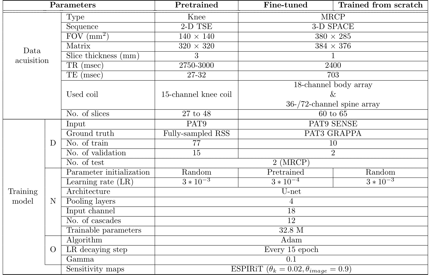
Tabel 1 Summary of three different model settings. The
Input for both DL models is SENSE reconstructed k-space on
PAT9. The test set for pertaining was used as the same PAT9 MRCP test set as other models. Different parameters between two DL models are initialized parameters and learning rates. D = Data, N =
Network, O = Optimizer
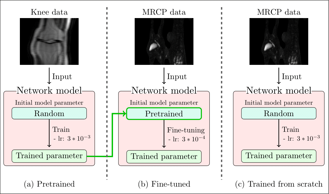
Figure 1 Overview of three types of models. (a) the
pretrained model takes the knee data as the input and learns randomly
initialized model parameters with a learning rate (lr) of 3*10-3. The model (b) initializes its parameters with
trained parameters of (a) to fine-tune them with a lower learning rate of 3*10-4. The model (c) optimizes parameters from
scratch with a learning rate of 3*10-3. Both (b) and (c) are trained with MRCP data.
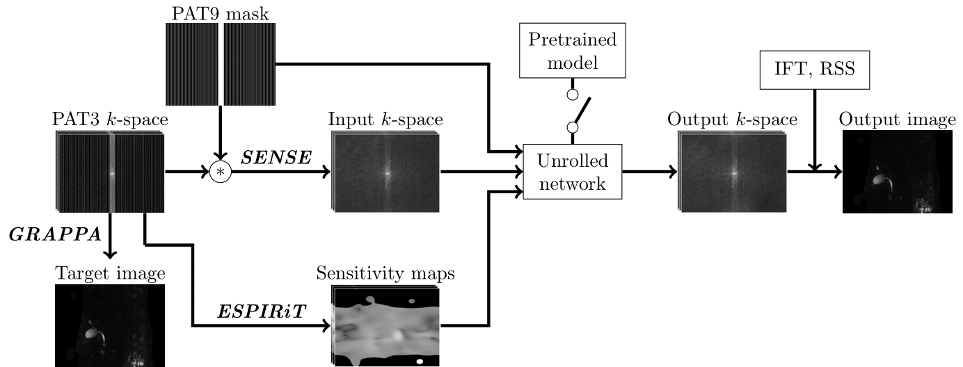
Figure 2 Pipeline of the DL-based MRCP reconstruction model. The input k-space is SENSE reconstructed k-space on retrospectively undersampled PAT9 k-space. The same sensitivity maps are used for SENSE and the unrolled network. The unrolled network architecture is the same as the VN. For fine-tuning, the pretrained model switch is on to initialize the parameters of the fine-tuned model with the pretrained parameters.
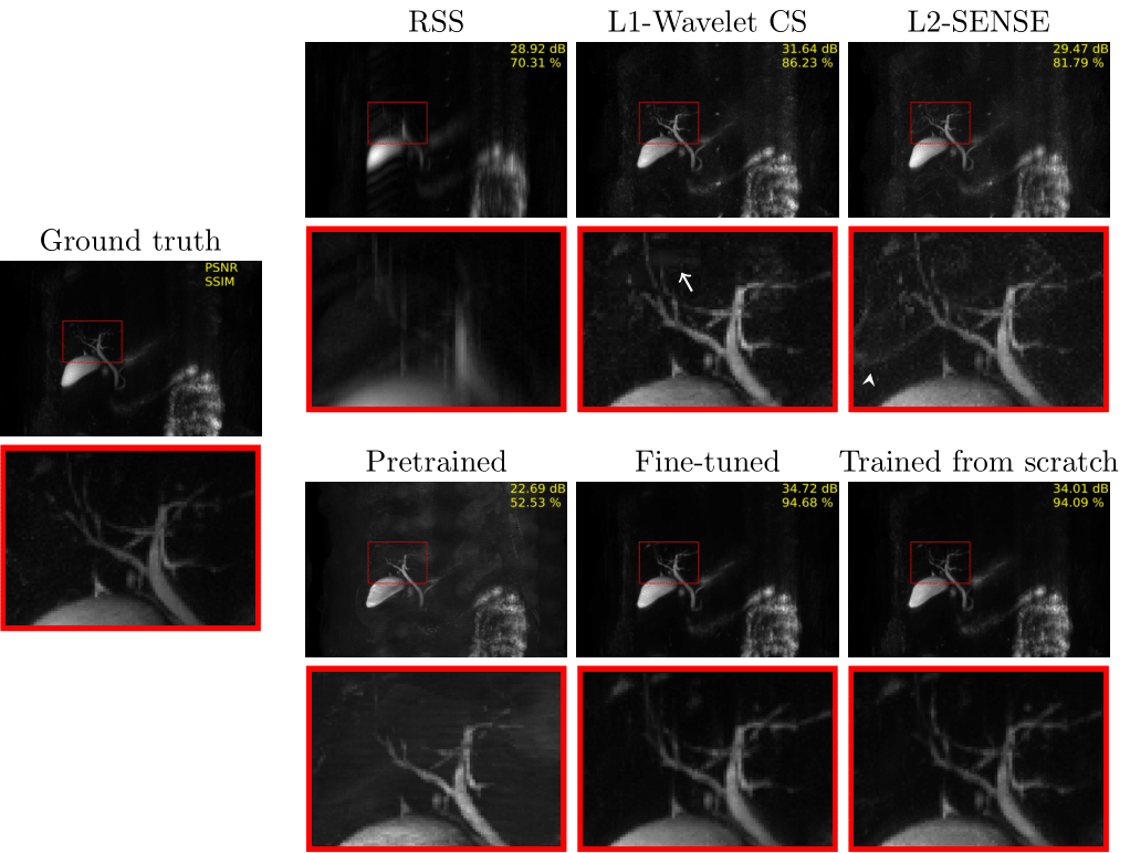
Figure 3 MIP images of each method applied on PAT9 MRCP
with corresponding zoom-ins (red boxes). A white arrow indicates wavelet compression artifacts in L1-Wavelet CS, and a white arrowhead points to where
aliasing artifacts mimicking ducts are seen in L2-SENSE.
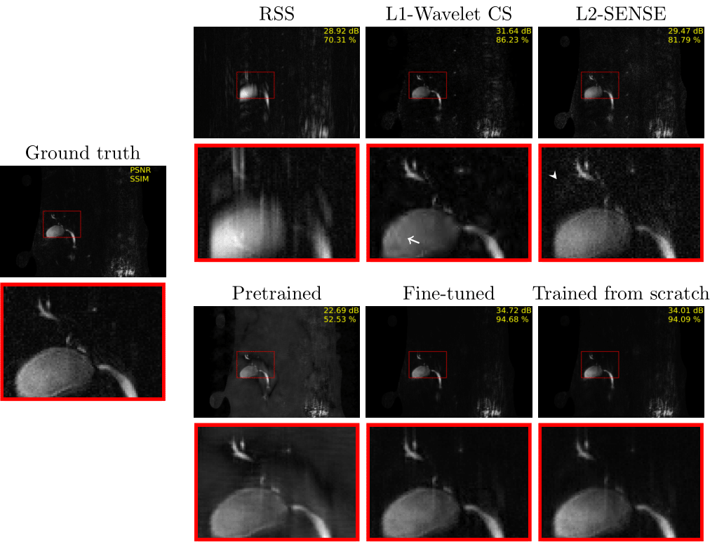
Figure 4 PAT9 MRCP single-slice images for each method. A white
arrow indicates wavelet compression artifacts in L1-wavelet CS. Moreover, a white arrowhead points
to where aliasing artifacts are seen in L2-SENSE.
DOI: https://doi.org/10.58530/2023/4777