4776

A Stochastic Approach for Joint Learning of a Neural Network Reconstruction and Sampling Pattern in Cartesian 3D Parallel MRI

Marcelo V. W. Zibetti¹ and Ravinder R. Regatte¹
¹Radiology, NYU Grossman School of Medicine, New York, NY, United States

Synopsis

Keywords: Data Acquisition, Image Reconstruction

This work proposes a stochastic variation of the bias-accelerated subset selection (BASS) algorithm to learn an efficient sampling pattern (SP) for accelerated MRI. This algorithm is used in the joint learning of an SP and neural network reconstruction. We apply the proposed approach to two different 3D Cartesian parallel MRI problems. The proposed stochastic approach, when used for joint learning, improves the learning speed from 2.5X to 5X, obtaining SPs with similar properties as the non-stochastic approach with nearly the same RMSE and SSIM.

Introduction:

One effective way to accelerate MRI is to acquire undersampled k-space data and combine it with special reconstructions (1–4). Undersampling has been used since partial Fourier acquisitions (5) and is commonly used, particularly in parallel MRI (6,7). Recently, deep learning image reconstructions have shown that neural networks (NN), such as the variational networks (VN) (8), can be even more effective in removing artifacts from undersampled images (3,8,9). However, no specific properties for the sampling pattern (SP) are currently known to be more or less effective with NN reconstruction. Several approaches have been proposed to jointly learn the SP and the NN (10–12), as an attempt to understand what are the sampling requirements for effective reconstruction with NN.
One effective approach for this joint learning problem is the alternated learning of NN reconstruction and SP (13), where ADAM (14) is used to learn the NN parameters, and bias-accelerated subset selection (BASS) (15) to learn the SP. The approach in (13), however, can be slow with large datasets because BASS uses all the images of the dataset in each iteration. Here, we proposed a stochastic version for BASS, that uses only part of the data at each iteration, resulting in much faster learning.

Methods:

A NN reconstruction can be written as
$$\hat{\mathbf{x}}=R_{\theta}(\bar{\mathbf{m}}, Ω),$$
where $$$R_{\theta}$$$ represents the NN with parameters $$$\theta$$$. We assume the following image-to-k-space model is used: $$$\mathbf{m}=\mathbf{FC}\mathbf{x}$$$, where $$$\mathbf{x}$$$ represents the 2D+time images, of size $$$N_x\times N_y \times N_t$$$ which denotes vertical $$$N_x$$$ and horizontal $$$N_y$$$ sizes and time $$$N_t$$$. $$$\mathbf{m}$$$ is the fully-sampled multi-coil k-t-space data. $$$\mathbf{C}$$$ denotes the coil sensitivities transform, which maps $$$\mathbf{x}$$$ into multi-coil weighted images of size $$$N_x \times N_y \times N_t \times N_c$$$, with number of coils $$$N_c$$$. $$$\mathbf{F}$$$ represents the spatial FFTs, which are $$$N_t \times N_c$$$ repetitions of the 2D-FFT.
When undersampled is used, then
$$\bar{\mathbf{m}}=\mathbf{S}_Ω\mathbf{FC}\mathbf{x},$$
where $$$\mathbf{S}_Ω $$$ is the sampling function using SP $$$Ω$$$ (same for all coils). The SP contains $$$M$$$ the k-t-space positions that will be sampled from a total of $$$N=N_x \times N_y \times N_t$$$ possible positions. The acceleration factor (AF) is defined as $$$N/M$$$.
The alternating approach from (13), formulates the joint learning problem as
$$Ω_{m+1}=\arg\min_{\begin{array}{c}Ω \subset \Gamma\\ s.t. |Ω|=M\end{array}} \frac{1}{N_i} \sum_{i=1}^{N_i}f(\mathbf{x}_i,R_{\theta_m}( \mathbf{S}_Ω\mathbf{FC}\mathbf{x}_i, Ω)),$$
$$\theta_{m+1}=\arg\min_{\theta \in \Theta}\frac{1}{N_i}\sum_{i=1}^{N_i}f(\mathbf{x}_i, R_{\theta}(\mathbf{S}_{Ω_{m+1}}\mathbf{FC}\mathbf{x}_i, Ω_{m+1})).$$
In the equations above, $$$N_i$$$ is the number of images used for training.
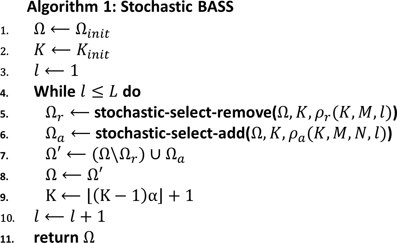
In (13), to learn the SP, some iterations of BASS (15) are used, but they can be time-consuming. Here we proposed a stochastic version of BASS, where only a small fraction of the data is used in the functions stochastic-select-remove and stochastic-select-add, described in Algorithm 1.
In this work, we compare the learning speed of BASS and the stochastic BASS ($$$K_{init}=1200$$$, $$$\alpha=0.75$$$, and stops when $$$L=31$$$, batch size of stochastic BASS is $$$16$$$ images), when used in the alternating learning, assuming a VN is jointly trained with ADAM (14) ($$$8$$$ epochs with initial learning-rate of $$$2\times10^{-4}$$$, with a learning-rate drop factor of $$$0.25$$$, applied every $$$2$$$ epochs, and batch size of $$$8$$$ images). Non-monotone versions of both algorithms are used.
We assessed the root mean squared error (RMSE) and structural similarity (SSIM) on two datasets: brain and knee. The brain dataset contains $$$750$$$ images of size $$$N=320 \times 320 \times 1$$$ for training, 50 for validation and $$$15$$$ for testing. The knee dataset contains $$$475$$$ images of size $$$N=256 \times 64 \times 2$$$ for training, $$$25$$$ for validation and $$$15$$$ for testing that are used for T1ρ mapping (16,17).

Results and Discussion:

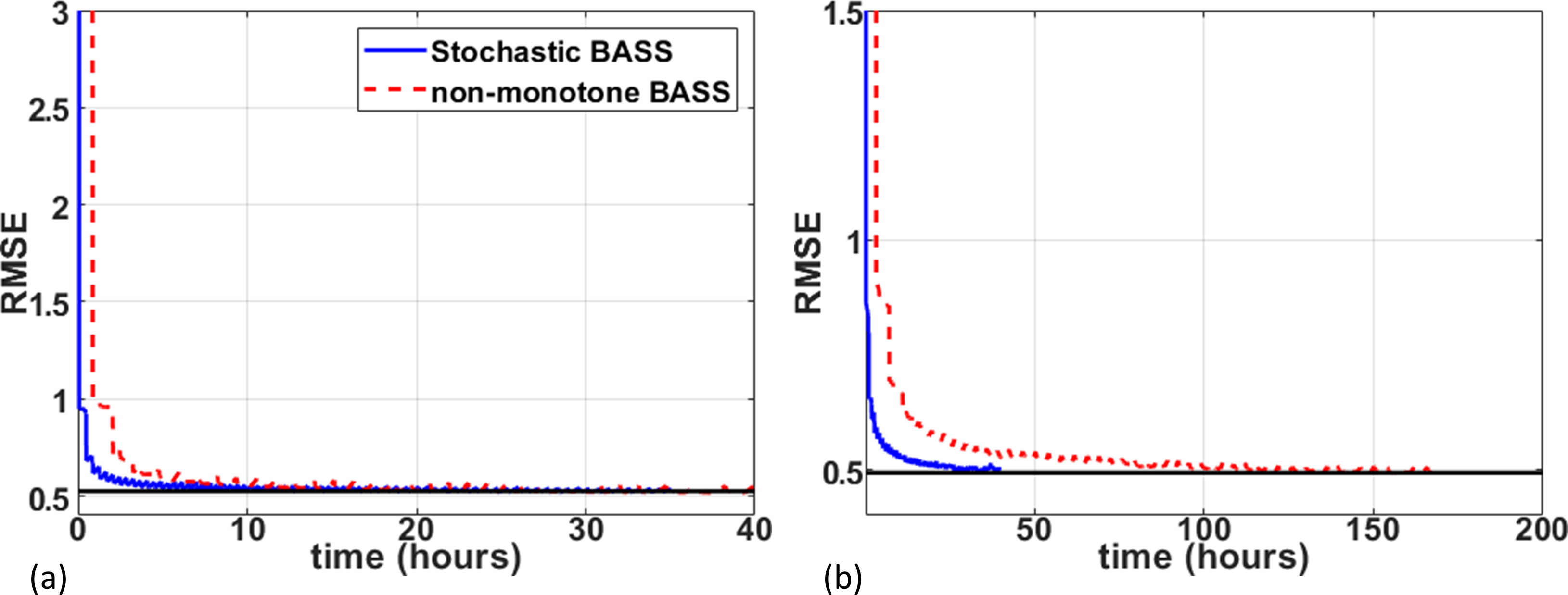
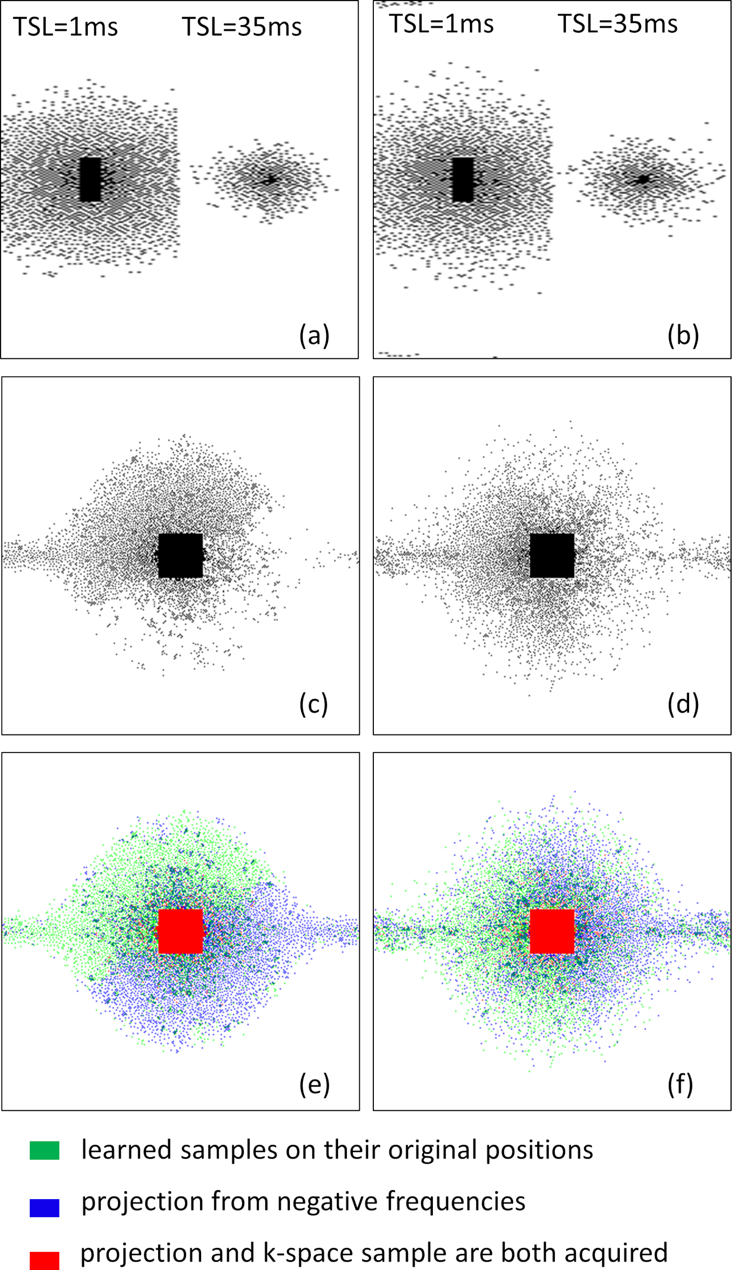
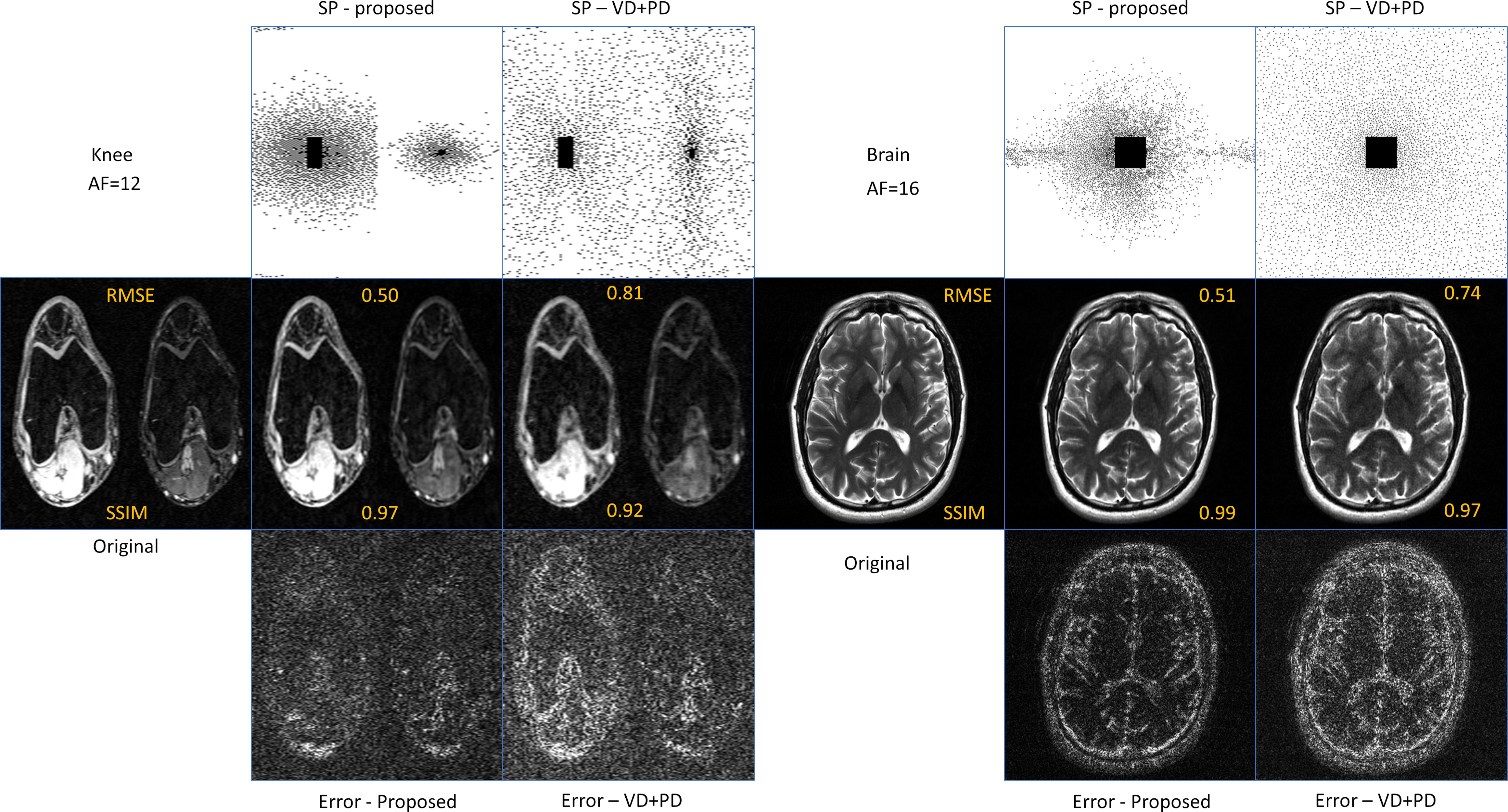
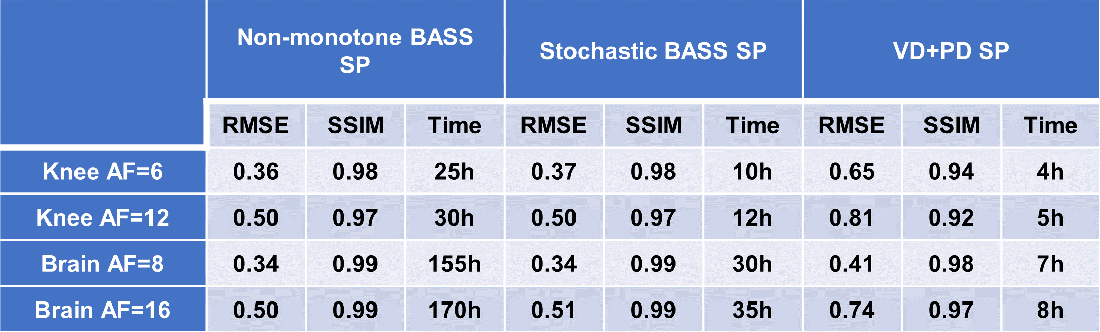
In Fig. 1 the resulting RMSE of the validation data along the training time is shown. This illustrates the learning speed of the algorithms. Essentially, the stochastic version reduced the training time by 5X times with datasets of this size. In Fig. 2 we observe some of the SPs learned by both methods. The stochastic version learned very similar SPs as BASS. In Table 1 we see the numerical results when compared to variable density and Poisson-disc SP (VD+PD SP). In Fig. 3 Some visual results comparing the proposed approach with a NN learned with VD+PD SP are shown.

Conclusion:

The proposed stochastic approach, when used for joint learning, improved the learning speed from 2.5X to 5X. The properties of the SPs learned by the algorithm and the quality of the images are similar to the non-stochastic version.

Acknowledgements

This study was supported by NIH grants, R21-AR075259-01A1, R01-AR068966, R01-AR076328-01A1, R01-AR076985-01A1, and R01-AR078308-01A1 and was performed under the rubric of the Center of Advanced Imaging Innovation and Research (CAI2R), an NIBIB Biomedical Technology Resource Center (NIH P41-EB017183).

References

1. Tamir JI, Ong F, Anand S, Karasan E, Wang K, Lustig M. Computational MRI With Physics-Based Constraints: Application to Multicontrast and Quantitative Imaging. IEEE Signal Process. Mag. 2020;37:94–104 doi: 10.1109/MSP.2019.2940062.

2. Feng L, Benkert T, Block KT, Sodickson DK, Otazo R, Chandarana H. Compressed sensing for body MRI. J. Magn. Reson. Imaging 2017;45:966–987 doi: 10.1002/jmri.25547.

3. Knoll F, Hammernik K, Zhang C, et al. Deep-learning methods for parallel magnetic resonance imaging reconstruction: A survey of the current approaches, trends, and issues. IEEE Signal Process. Mag. 2020;37:128–140 doi: 10.1109/MSP.2019.2950640.

4. Jacob M, Ye JC, Ying L, Doneva M. Computational MRI: Compressive Sensing and Beyond [From the Guest Editors]. IEEE Signal Process. Mag. 2020;37:21–23 doi: 10.1109/MSP.2019.2953993.

5. Liang ZP, Lauterbur PC. Principles of magnetic resonance imaging: a signal processing perspective. IEEE Press; 2000.

6. Ying L, Liang Z-P. Parallel MRI Using Phased Array Coils. IEEE Signal Process. Mag. 2010;27:90–98 doi: 10.1109/MSP.2010.936731. 7. Blaimer M, Breuer F, Mueller M, Heidemann RM, Griswold MA, Jakob PM. SMASH, SENSE, PILS, GRAPPA. Top. Magn. Reson. Imaging 2004;15:223–236 doi: 10.1097/01.rmr.0000136558.09801.dd.

8. Hammernik K, Klatzer T, Kobler E, et al. Learning a variational network for reconstruction of accelerated MRI data. Magn. Reson. Med. 2018;79:3055–3071 doi: 10.1002/mrm.26977.

9. Liang D, Cheng J, Ke Z, Ying L. Deep magnetic resonance image reconstruction: Inverse problems meet neural networks. IEEE Signal Process. Mag. 2020;37:141–151 doi: 10.1109/MSP.2019.2950557.

10. Bahadir CD, Wang AQ, Dalca A V., Sabuncu MR. Deep-Learning-Based Optimization of the Under-Sampling Pattern in MRI. IEEE Trans. Comput. Imaging 2020;6:1139–1152 doi: 10.1109/TCI.2020.3006727.

11. Aggarwal HK, Jacob M. J-MoDL: Joint Model-Based Deep Learning for Optimized Sampling and Reconstruction. IEEE J. Sel. Top. Signal Process. 2020;14:1151–1162 doi: 10.1109/JSTSP.2020.3004094.

12. Weiss T, Vedula S, Senouf O, Michailovich O, Zibulevsky M, Bronstein A. Joint Learning of Cartesian under Sampling and Reconstruction for Accelerated MRI. In: IEEE International Conference on Acoustics, Speech and Signal Processing. Vol. 2020–May. IEEE; 2020. pp. 8653–8657. doi: 10.1109/ICASSP40776.2020.9054542.

13. Zibetti MVW, Knoll F, Regatte RR. Alternating Learning Approach for Variational Networks and Undersampling Pattern in Parallel MRI Applications. IEEE Trans. Comput. Imaging 2022;8:449–461 doi: 10.1109/TCI.2022.3176129.

14. Kingma DP, Ba J. Adam: A Method for Stochastic Optimization. arXiv Prepr. 2014:1–15.

15. Zibetti MVW, Herman GT, Regatte RR. Fast data-driven learning of parallel MRI sampling patterns for large scale problems. Sci. Rep. 2021;11:19312 doi: 10.1038/s41598-021-97995-w.

16. Zibetti MVW, Sharafi A, Otazo R, Regatte RR. Accelerating 3D-T1ρ mapping of cartilage using compressed sensing with different sparse and low rank models. Magn. Reson. Med. 2018;80:1475–1491 doi: 10.1002/mrm.27138.

17. Zibetti MVW, Johnson PM, Sharafi A, Hammernik K, Knoll F, Regatte RR. Rapid mono and biexponential 3D-T1ρ mapping of knee cartilage using variational networks. Sci. Rep. 2020;10:19144 doi: 10.1038/s41598-020-76126-x.

Figures

Algorithm 1: Stochastic BASS

Fig. 1: Resulting RMSE of the validation data along the training time for (a) knee, at AF=12, and (b) brain, at AF=16, datasets. This illustrates the learning speed of the algorithms. Essentially, the stochastic version reduced the training time from 2.5X (knee) to 5X (brain) with the tested datasets.

Fig. 2: In this figure, we can notice the difference in the SPs learned with the knee dataset (AF=12) by (a) BASS and (b) stochastic BASS. We can notice the variable sampling density over time, resampling the low-frequency components as in Keyhole methods. The SPs learned with the brain dataset (c) for BASS and (d) stochastic BASS are even more interesting. The gaps where samples are missing are filled by the complex-conjugated positions, seen in (e) and (f), as in partial Fourier acquisitions. One can also notice variable density and spacing between samples as in Poisson-disc SPs.

Fig.3: In this figure, we can visually see the improvement of the images (results of BASS are not shown since they are nearly identical to the proposed approach) with knee and brain datasets. The visual improvement when compared to VD+PD SPs can be easily seen at these acceleration factors.

Table 1. RMSE, SSIM, and training time for both datasets using testing images.

Proc. Intl. Soc. Mag. Reson. Med. 31 (2023)

4776

DOI: https://doi.org/10.58530/2023/4776