4772
Deep learning-based Lorentzian fitting of WASSR Z-spectra
1Medical Physics, Lund University, Lund, Sweden, 2Radiology, F.M. Kirby Research Center, Johns Hopkins University, Kennedy Krieger Institute, Baltimore, MD, United States, 3Radiology, Johns Hopkins University, Baltimore, MD, United States, 4F.M. Kirby Research Center, Radiology, Medical Radiation Physics, Kennedy Krieger Institute, Johns Hopkins University, Lund University, Baltimore, MD, United States
Synopsis
Keywords: Data Analysis, Machine Learning/Artificial Intelligence, Lorentzian curve fitting
Water saturation shift referencing (WASSR) Z-spectra can be used to correct shifts due to B0-field inhomogeneities, for magnetic susceptibility mapping and analysis of relaxation effects. The spectra follow a Lorentzian shape with discrete values. Hence, a Lorentzian fit to retrieve the shape parameters (amplitude A, line width LW and frequency shift ΔfH2O ) simplifies analysis. Conventionally, the least-squares (LS) method is used for such fitting despite being time consuming and sensitive to the unavoidable noise in vivo. We propose a deep learning-based Lorentzian-fitting neural network (LoFNet) that demonstrated improved robustness against noise and sampling density in combination with reduced time consumption.Introduction
By irradiating a sample with radiofrequency (RF) pulses over a discrete number of offset frequencies and taking the normalized water signal as a function of the saturation frequencies a Z-spectra is formed6. If the irradiated sample contains exchangeable protons in solute molecules the water signal in the Z-spectrum will decrease at the resonance frequency of the solute due to saturation transfer1,6–11. At the resonance frequency of water, the signal will be further reduced due to direct saturation (DS)6 which will result in a Lorentzian shape12. By using a sufficiently low B1 and short saturation duration the DS effect in the Z-spectrum can be isolated1 yielding a water saturation shift referencing (WASSR) Z-spectrum. WASSR Z-spectra are useful for correcting shifts due to B0-field inhomogeneities1–4, for magnetic susceptibility mapping5 and analysis of relaxation effects4. By fitting a WASSR Z-spectrum to a Lorentzian curve, the shape parameters (amplitude A, line width LW and frequency shift $$$\Delta f_{H_2O}$$$) are directly obtained thus simplifying the analysis. The conventional approach is to use a least-squares Lorentzian fitting. However, this method is time consuming and sensitive to the unavoidable in vivo noise. To overcome these shortcomings, we propose to use a deep learning based Lorentzian fitting neural network (LoFNet).Theory
The normalized WASSR Z-spectrum follows a Lorentzian line shape defined as:$$Z(\Delta f_{RF})=\frac{S_{sat}(\Delta f_{RF})}{S_0}=1-\frac{A\cdot LW^2}{LW^2+4(\Delta f_{RF}-\Delta f_{H_2O})} (1)$$
where $$$S_{sat}(\Delta f_{RF})$$$ is the signal intensity at the irradiation offset from the water proton frequency, $$$S_0$$$ is the intensity without saturation and $$$\Delta f_{RF}$$$ is the saturation frequency offset (in Hz). A is the normalized signal amplitude, LW the linewidth (in Hz) and $$$\Delta f_{H_2O}$$$ is the water proton frequency offset (in Hz).
Methods
A training dataset consisting of 5,000,000 sample-label pairs was simulated using Eq. (1) and noise was added before transforming each sample to be governed by a Rician probability density function. The shape parameters (A, LW and $$$\Delta f_{H_2O}$$$) were randomly chosen from pre-defined intervals for each sample and saved as a corresponding label to the simulated sample. Similarly, a test dataset was simulated consisting of 10,000 sample-label pairs. An additional group of test data was simulated each with 10,000 sample-label pairs but with increasing noise level from 0 to 4.5 % with 0.5 % increments. The study was approved by the Institutional Review Board (IRB) and written informed consent was obtained from each subject. WASSR Z-spectra from 3 T scans were extracted from white matter (WM), gray matter (GM), cerebrospinal fluid (CSF) and tumour (T) regions yielding in vivo datasets. A neural network architecture was constructed and the hyperparameters optimized using the Python library HyperOpt13. The optimized network LoFNetHP was trained on 90 % of the training dataset and the remaining part was used as a validation set during training. The trained model was evaluated on the in vivo and simulated datasets. Prediction errors (PEs), robustness against increased noise and robustness against reduced sampling density were compared to those of the LS-method. In addition, a comparison of the time consumption for the two methods was made. Metrics used were root-mean-squared error (RSME) and mean-absolute error (MAE).Results
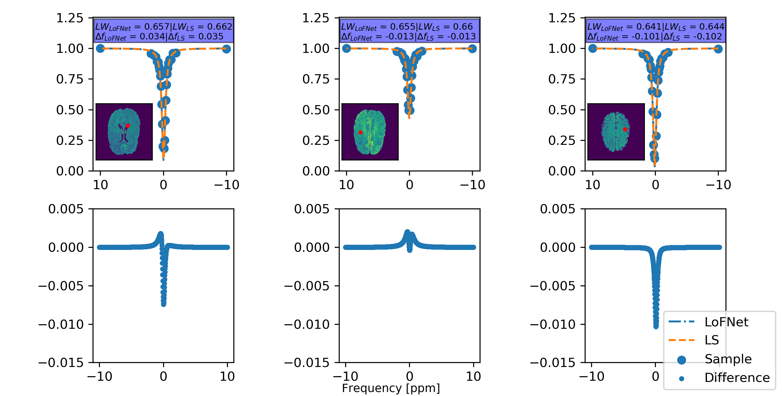
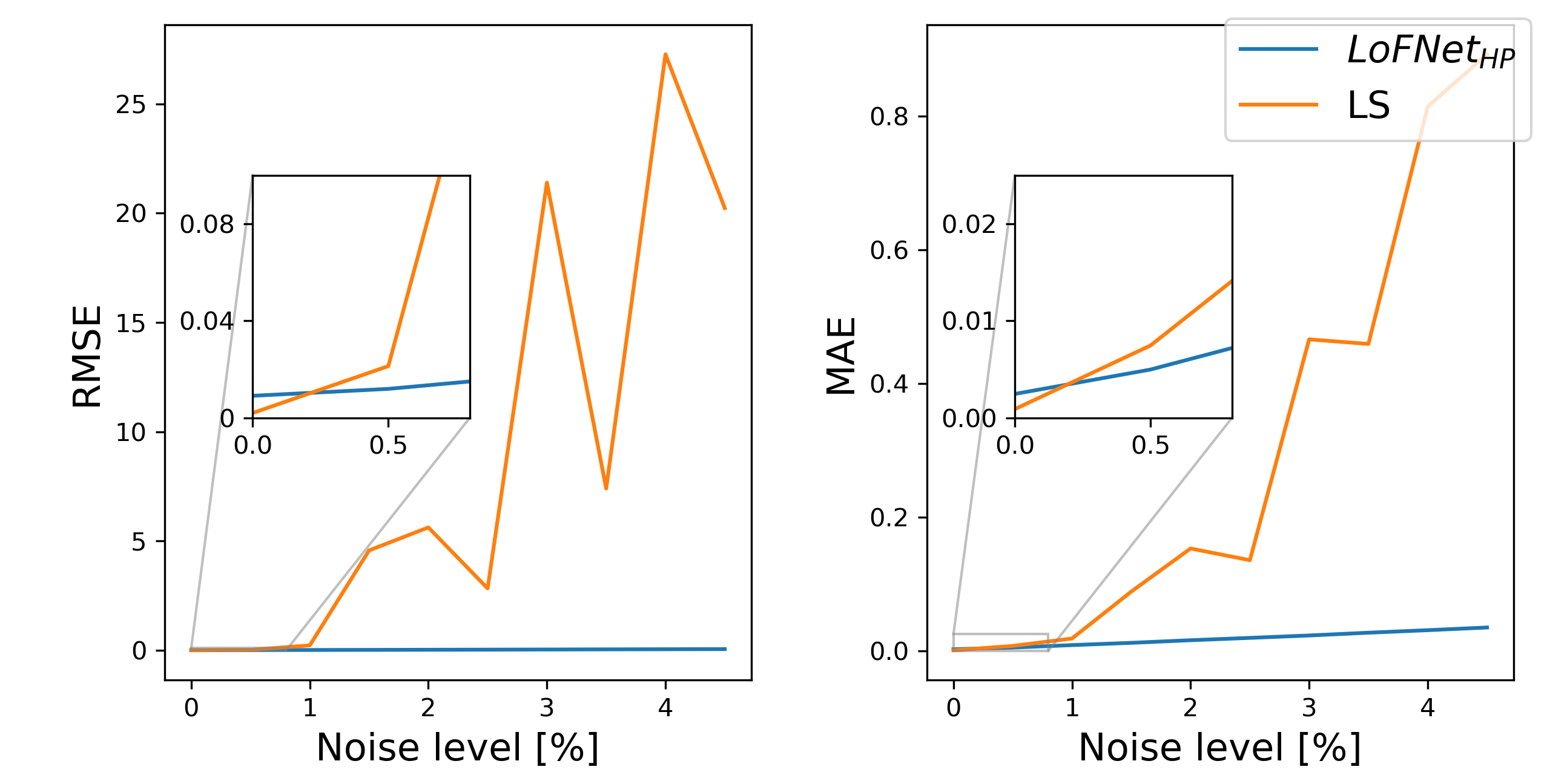
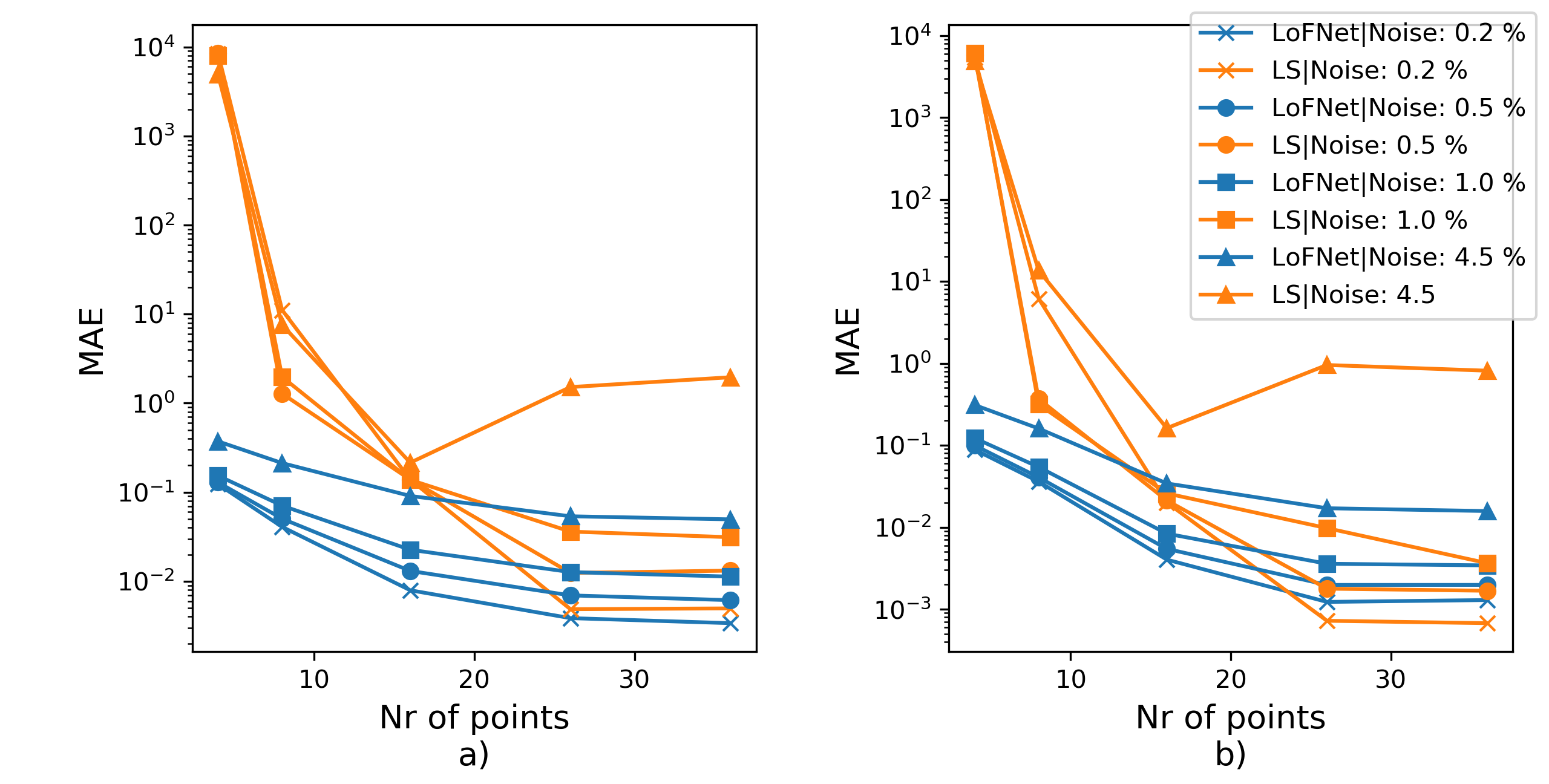
The LoFNetHP and the LS-method produced comparable PEs on all in vivo datasets (WM, GM, CSF, T) with no statistically significant difference $$$p=0.35$$$ and $$$p=0.27$$$ for RMSE and MAE, respectively. Figure 1 shows three representative fits on samples from WM, GM, and CSF. Both methods showed good fits to the discrete sample values and are overlapped by visual inspection. A closer analysis (Figure 1, bottom row) shows small differences between the two methods on the order of 1 % or less. However, a significant difference ($$$p=0.048$$$) in time consumption was observed, where LoFNetHP was on average 70 times faster.The LS-method exhibited a tendency of a rapid increase in PEs with increased sample noise (same trend can be seen for both metrics), whereas LoFNetHP showed marginal increase of PE up to 4.5 % (Figure 2). The insets of Figure 2 show that the PEs for LS start to increase after 0.5 %. The two methods produced comparable PEs up to approximately 1 % after which the PEs for LS took off rapidly. With reduced number of sample points, the PEs increased for both methods (Figure 3). However, the increase occurred earlier and is more pronounced for LS.
Discussion
The improved robustness against noise for LoFNetHP compared to LS allows for higher noise levels and thus a reduced MRI acquisition time of the WASSR spectra or alternatively, an increased spatial resolution. This can be applied to, for example, quantitative susceptibility mapping. The improved robustness of LoFNetHP against reduced sampling density compared to LS is a good indicator of the method’s generalizability to different sampling protocols. However, the sampling density should not be reduced below 8 points to ensure sufficiently low PEs (Figure 3).Conclusion
In Lorentzian fitting of WASSR spectra, the proposed deep learning method, LoFNetHP, showed improved robustness against noise and against reduced sampling density as well as significantly reduced time consumption compared to the conventional LS-method. These advantages increase the efficiency of the analysis, ease SNR requirements and facilitate generalizability.Acknowledgements
No acknowledgement found.References
1. Kim M, Gillen J, Landman BA, Zhou J, van Zijl PCM. Water saturation shift referencing (WASSR) for chemical exchange saturation transfer (CEST) experiments. Magn Reson Med. 2009;61(6):1441-1450. doi:10.1002/mrm.21873
2. Müller-Lutz A, Matuschke F, Schleich C, et al. Improvement of water saturation shift referencing by sequence and analysis optimization to enhance chemical exchange saturation transfer imaging. Magn Reson Imaging. 2016;34(6):771-778. doi:10.1016/j.mri.2016.03.013
3. Liu G, Qin Q, Chan KWY, et al. Non-invasive temperature mapping using temperature-responsive water saturation shift referencing (T-WASSR) MRI. NMR Biomed. 2014;27(3):320-331. doi:10.1002/nbm.3066
4. Smith SA, Bulte JWM, van Zijl PCM. Direct saturation MRI: theory and application to imaging brain iron. Magn Reson Med. 2009;62(2):384-393. doi:10.1002/mrm.21980
5. Lim IAL, Li X, Jones CK, Farrell JAD, Vikram DS, van Zijl PCM. Quantitative magnetic susceptibility mapping without phase unwrapping using WASSR. NeuroImage. 2014;86:265-279. doi:10.1016/j.neuroimage.2013.09.072
6. van Zijl PCM, Yadav NN. Chemical exchange saturation transfer (CEST): what is in a name and what isn’t? Magn Reson Med. 2011;65(4):927-948. doi:10.1002/mrm.22761
7. Zhou J, Payen JF, Wilson DA, Traystman RJ, van Zijl PCM. Using the amide proton signals of intracellular proteins and peptides to detect pH effects in MRI. Nat Med. 2003;9(8):1085-1090. doi:10.1038/nm907
8. Gilad AA, McMahon MT, Walczak P, et al. Artificial reporter gene providing MRI contrast based on proton exchange. Nat Biotechnol. 2007;25(2):217-219. doi:10.1038/nbt1277
9. van Zijl PCM, Jones CK, Ren J, Malloy CR, Sherry AD. MRI detection of glycogen in vivo by using chemical exchange saturation transfer imaging (glycoCEST). Proc Natl Acad Sci U S A. 2007;104(11):4359-4364. doi:10.1073/pnas.0700281104
10. Ward KM, Aletras AH, Balaban RS. A new class of contrast agents for MRI based on proton chemical exchange dependent saturation transfer (CEST). J Magn Reson San Diego Calif 1997. 2000;143(1):79-87. doi:10.1006/jmre.1999.1956
11. Vinogradov E, Sherry AD, Lenkinski RE. CEST: from basic principles to applications, challenges and opportunities. J Magn Reson San Diego Calif 1997. 2013;229:155-172. doi:10.1016/j.jmr.2012.11.024
12. Mulkern RV, Williams ML. The general solution to the Bloch equation with constant rf and relaxation terms: application to saturation and slice selection. Med Phys. 1993;20(1):5-13. doi:10.1118/1.597063
13. Bergstra J, Yamins D, Cox D. Hyperopt: A Python Library for Optimizing the Hyperparameters of Machine Learning Algorithms.; 2013:19. doi:10.25080/Majora-8b375195-003
Figures