4727
Quantitative sodium MRI of the human kidneys at 7T – Before, during and after water load via sliding window evaluation1Medical Physics in Radiology, German Cancer Research Center (DKFZ), Heidelberg, Germany, 2Faculty of Physics and Astronomy, Heidelberg University, Heidelberg, Germany, 3University Hospital Erlangen, Institute of Radiology, Friedrich‐Alexander‐Universität Erlangen‐Nürnberg (FAU), Erlangen, Germany, 4Faculty of Medicine, Heidelberg University, Heidelberg, Germany
Synopsis
Keywords: Non-Proton, High-Field MRI, Kidney, Quantitative Imaging
23Na-MRI is a non-invasive tool for the in-vivo quantification of the tissue sodium concentration (TSC); however, it suffers from low in-vivo signals and short relaxation times. High magnetic field strengths, dedicated hardware and pulse sequences as well as various correction methods contribute to obtaining reliable TSCs. In the presented work we employ a custom-built coil and reference vial setup and perform T1, B1+ and B1- corrections that were validated in phantom measurements. We use a sliding window reconstruction for the quantitative 23Na-images to investigate the changes in the TSC before, during and after a water load in two healthy volunteers.
Introduction
Sodium (23Na) MRI of the human kidneys is a promising candidate for a non-invasive biomarker to assess renal tissue function and viability1, as the kidneys play a key role in maintaining the fluid and electrolyte homeostasis in the human body.In this work sliding window reconstruction of quantitative 23Na images is applied in two healthy volunteers to investigate the changes in the TSC not only after water deprivation and after the water load2, but also during and immediately after water uptake. T1, B1+ and B1- corrections are employed to get reliable tissue sodium concentration (TSC) values. These correction methods were first validated for the applied setup in phantom measurements3. Furthermore, we designed and built a fixed setup for the reference vials to ensure consistent placement within the coil and thus reduce the influence of manual evaluation and ensure consistency with the simulated B1- fields.
Methods
The TSC was determined in two healthy volunteers (female, age 27/32 years, weight 65/85 kg) measured head-first supine with the hands above the head.For the concentration determination, four external reference vials with NaCl solutions were positioned under the phantom (20mM, 30mM, 40mM, 50mM) or under the back of the volunteer (20mM, 60mM, 100mM, 140mM). The four reference vials were positioned in an interchangeable compartment filled with 35mM NaCl solution and 2% agarose within a fixed setup.
Sodium measurements were performed on a 7T whole-body MR system4 with a custom-built oval-shaped body coil5. For phantom investigations, a phantom filled with 35mM NaCl solution was measured. Density-adapted 3D radial sampling6 (DA-3DPR) with a golden angle projection distribution7 was applied. To generate B1+ maps, the dual flip angle method8 was used.
To achieve water deprivation, both volunteers abstained from drinking or eating at least 13 hours prior to the 23Na MRI. B1+ maps were measured first, followed by a 1h DA-3DPR measurement and an additional 15min DA-3DPR measurement. 20min into the 1h measurement, volunteer one and two drank 629ml and 1044ml out of a reservoir of approximately 1000ml of water (Na+: 20mg/l), respectively.
To correct for B1- inhomogeneities, B1- maps of the radiofrequency coil were simulated5 for the phantom setup as well as in a human voxel model9,10 (Ella, scaled by 5% to better fit the volunteers’ anatomy) using the electromagnetic field simulation software CST11. The B1+ maps were Gauss-filtered (σ=10mm), while the quantitative image data were filtered with a Hamming filter. The quantitative in-vivo images were zero-filled with a filling factor of two and the B1+ maps were zero-filled to generate the same voxel size as the quantitative images. T1 relaxation effects in the reference vials and phantom were corrected according to the FLASH equation. Quantitative images were reconstructed using a sliding window with 4500 projections per subset (7.5min duration). The concentrations in the phantom and kidneys were determined with a semi-automated segmentation tool self-developed in Matlab12 using the known concentration in the reference vials and a linear fit.
Results
For the phantom measurement the determined sodium concentrations converge to the ground truth after the corrections (see Fig. 2). In vivo measurements in volunteer one (see Fig. 3-5) yielded a TSC change from before to after the water load of (57.1±22.7)mM to (59.8±12.6)mM for the left and (67.5±17.5)mM to (56.5±9.9)mM for the right kidney. Furthermore, a decrease of the cortico-medullary sodium gradient was observed, as can be seen in the decreased standard deviation in Figure 4a. For volunteer two (see Fig. 3-5) a change of (51.8±11.7)mM to (53.8±11.6)mM and (54.9±10.3)mM to (56.7±9.5)mM was found for the left and right kidney, respectively.Discussion & Conclusion
The concentrations determined in the phantom validated the gain in accuracy provided by the correction methods for the presented setup and are visualized in Fig. 2.Data evaluation with a sliding window was successfully applied to 23Na MRI at 7T before, during and after a water load. As the human kidney contains different tissue types including cortex, medulla and renal pelvis13, the concentrations determined here are average values for the combination of these tissue types. Registration of the 23Na images with high-resolution hydrogen images would enable the segmentation of the different tissue compartments, thereby enabling a more accurate determination of the sodium concentration of each individual tissue type, but so far the setup does not allow for dual-nuclear 23Na/1H measurement without repositioning the volunteer. As the ROIs were drawn in the full data set, they might not fit as well for the left kidney of volunteer one where there was pronounced kidney movement after the water load (see Fig. 5). In future work, the ROIs will be adjusted to the subsets.
Interestingly, the decrease in TSC following a water load as described by, for example, Haneder et al.2 can only be observed for one of the volunteers. In addition to abstaining from food and drink for a period of time, other influences could be relevant such as general diet, fitness, or hormonal changes during the menstrual cycle14. These effects could be further investigated in future studies.
Nevertheless, the measured TSCs are in good agreement with the literature measurements conducted at 3T2, ranging from (48.6±5.3)mmol/L to (108.0±10.9)mmol/L depending on the physiologic condition and segmented tissue type.
Acknowledgements
No acknowledgement found.References
1. F. G. Zöllner et al. NMR Biomed. (2016). https://doi.org/10.1002/nbm.3274.
2. S. Haneder et al. Radiology (2011). https://doi.org/10.1148/radiol.11102263
3. A. Scheipers et al. Proc. Intl. Soc. Mag. Reson. Med. 30 (2021). Abstract: 0238.
4. MAGNETOM 7T, Siemens Healthcare GmbH, Erlangen, Germany
5. T. Platt et al. Magn. Reson. Med. (2018). https://doi.org/10.1002/mrm.27103
6. A. M. Nagel et al. Magn. Reson. Med. (2009). https://doi.org/10.1002/mrm.22157
7. R. W. Chan et al. Magn. Reson. Med. (2009). https://doi.org/10.1002/mrm.21837
8. E. K. Insko, L. Bolinger, J. Magn. Reson. (1993). https://doi.org/10.1006/jmra.1993.1133.
9. A. Christ et al. Phys. Med. Biol. (2010); 55:N23-N38.
10. P. A. Hasgall et al. IT’IS database for thermal and electromagnetic parameters of biological tissues, Version 2.6, www.itis.ethz.ch/database.
11. CST Studio Suite 2019/2020 (Dassault Systèmes, Vélizy-Villacoublay, France)
12. The MathWorks Inc., Natick, MA, USA
13. C. J. Lote, (2012), Principles of Renal Physiology, Springer, New York, https://doi.org/10.1007/978-1-4614-3785-7
14. A. Pechère-Bertschi et at. Kidney International (2002). https://doi.org/10.1046/j.1523-1755.2002.00158.xFigures
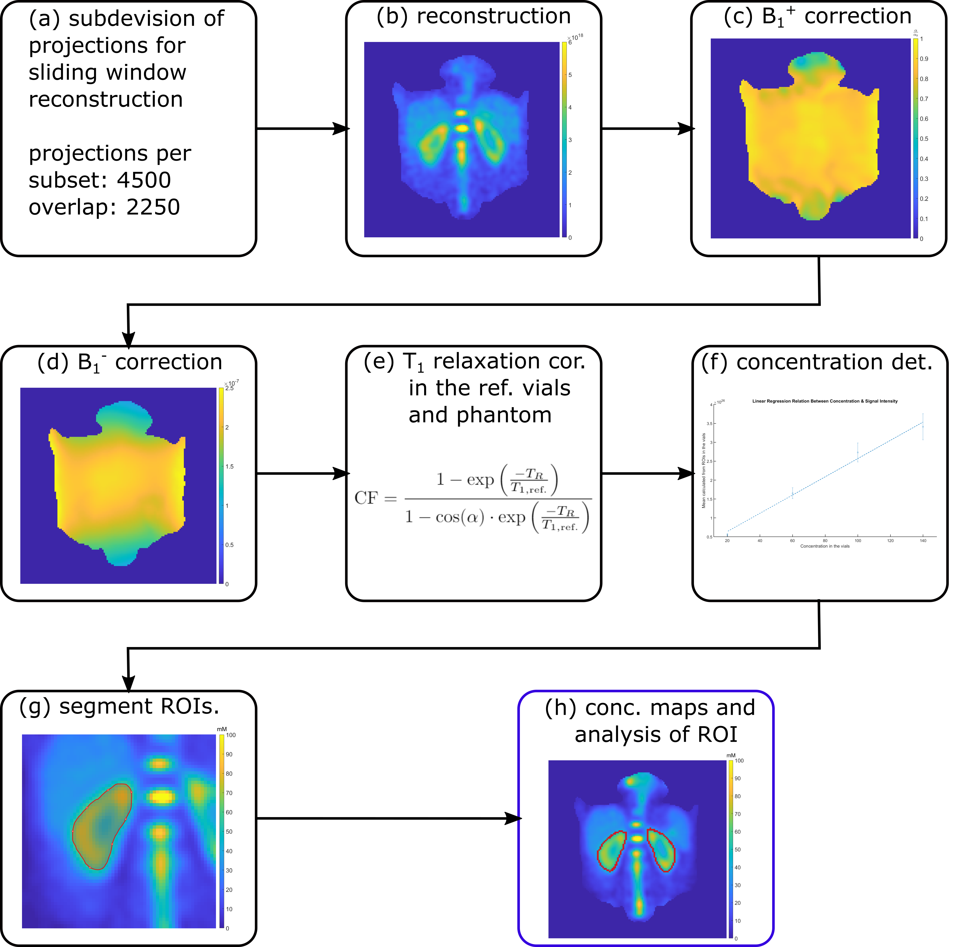
Fig. 1: A schematic of the workflow employed is depicted from the subdivision of the projections for sliding window reconstruction (a) to the determination of the sodium concentration in the kidneys (h). Quantitative images were acquired with the following parameters: flip angle α=61°, TE/TR=1ms/100ms, nominal spatial resolution (Δx)3=(6mm)3, pulse duration tP=1.8ms, readout time tRO=5ms, number of projections nProj=36000+9000. B1+ maps were acquired with the dual flip angle method7 (α=45°/90°, TE/TR=1.55ms/150ms, (∆x)3=(10mm)3, tP=3ms, tRO=10ms, nProj=4100).
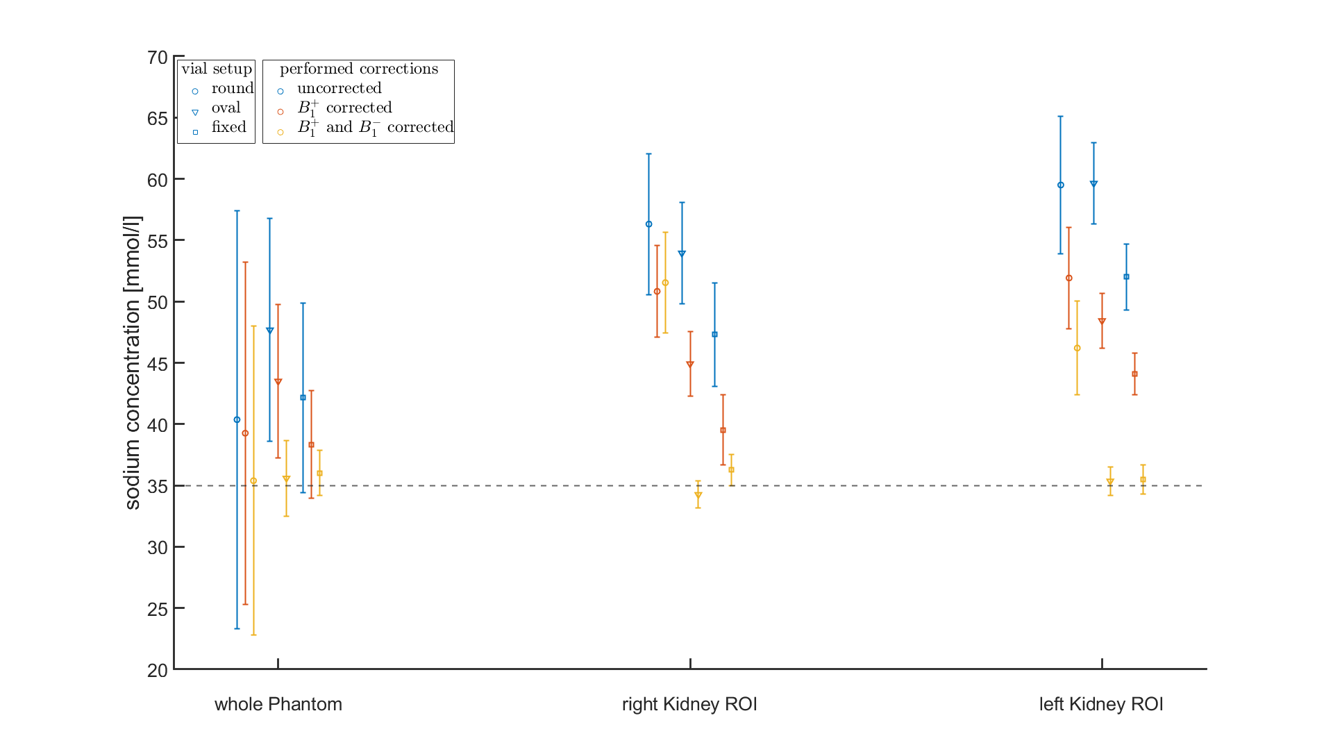
Fig. 2: Comparison of the phantom (35mM) measurements with the round and oval reference vials to the fixed setup, showing the concentrations for the data without correction as well as after B1+ field correction (measured B1+ map) and after both B1+ (measured) and B1- (simulated) correction. The concentration in the whole phantom ROI as well as in the evaluated kidney-emulating ROIs of the first measurement of Volunteer One are plotted. Due to the generally lower positioning of the phantom for the second and third setup, the evaluated ROIs were shifted to emulate the same position.
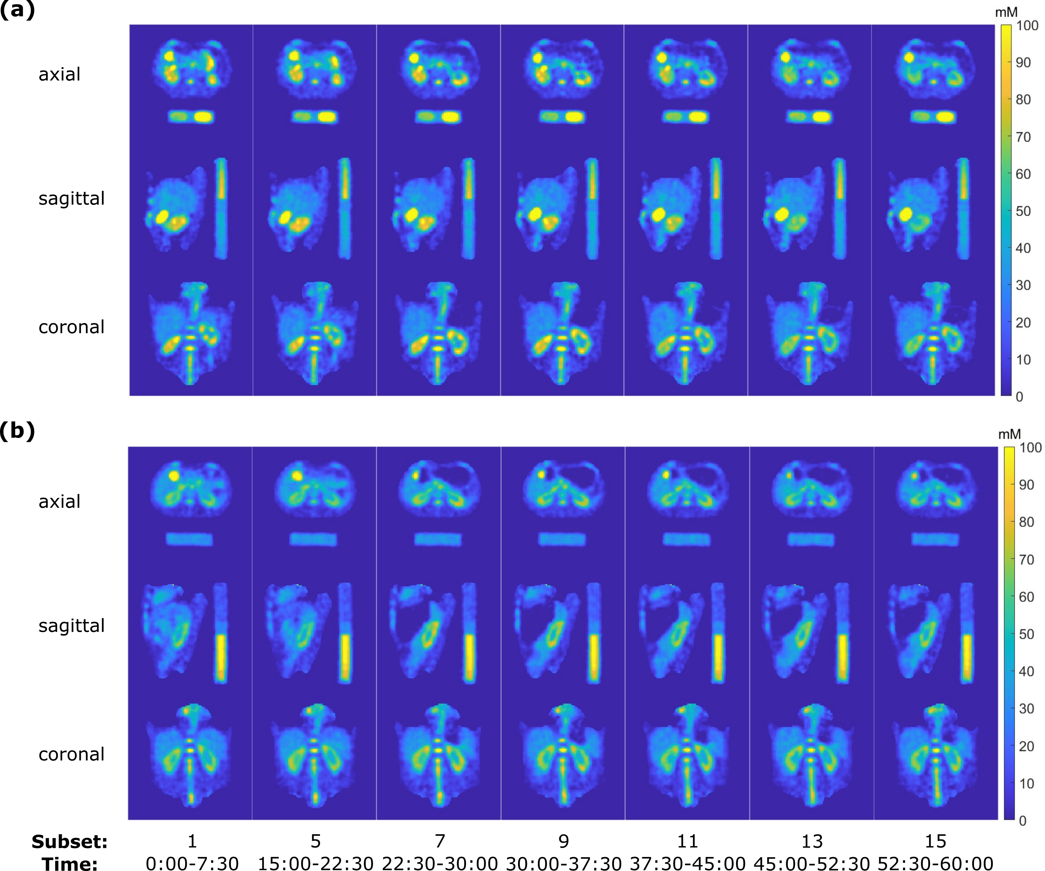
Fig. 3: Quantitative 23Na concentration in the human torso at 7T for volunteer one (a) and two (b) for a selection of the evaluated subsets during the 1h measurement. At t = 20min, volunteers one and two drank 629ml and 1044ml of water (Na+: 20mg/l) respectively. Slices in each orientation were chosen to visualize the kidneys.
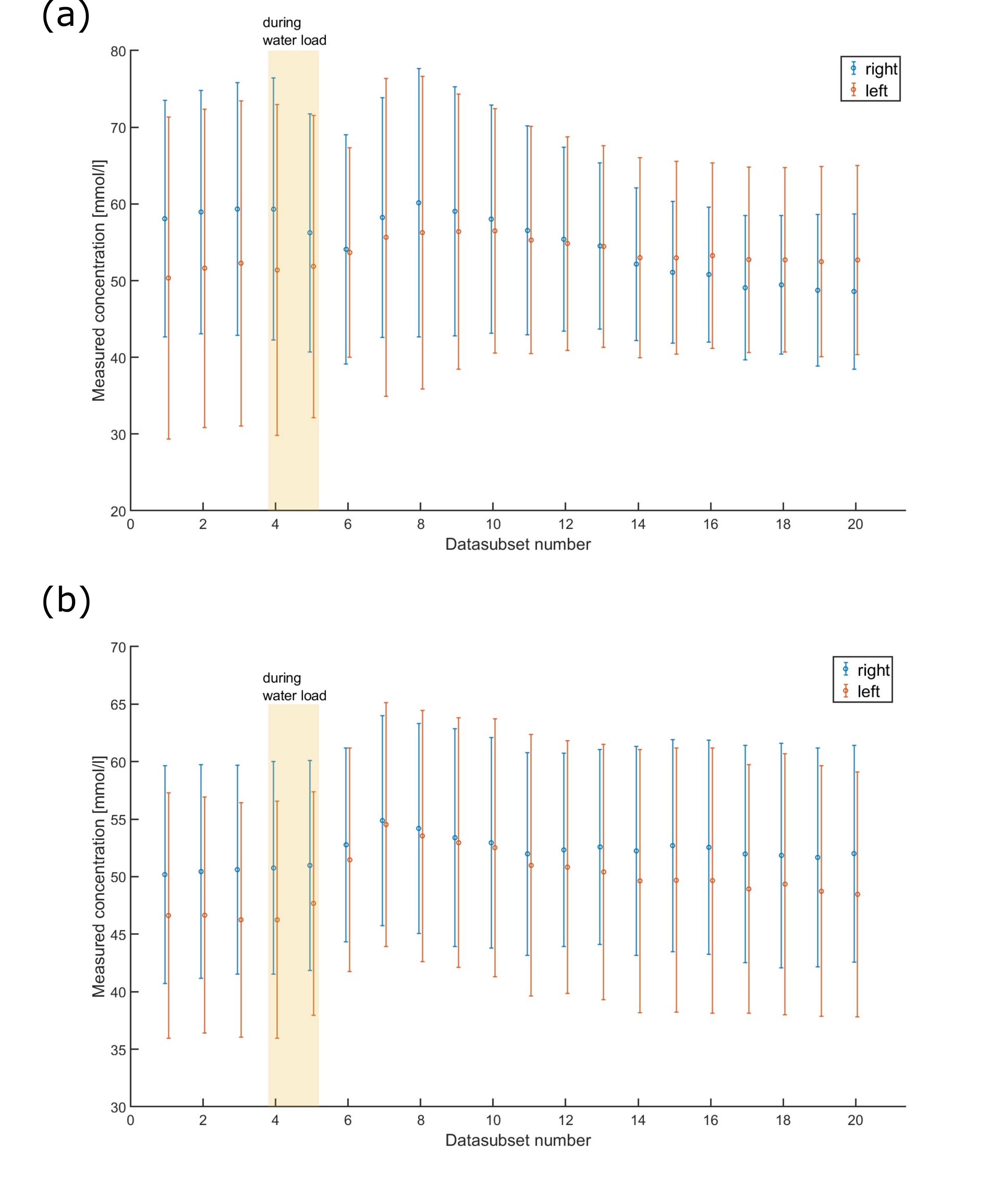
Fig. 4: Change in concentration in the left and right kidney of volunteer one (a) and two (b) after T1, B1+ and B1- corrections during the course of the 1h measurement. Each data subset has a length of 4500 projections, corresponding to a measurement time of 7.5min and an overlap of 2250 projections. At t = 20 min, volunteers one and two drank 629ml and 1044ml of water (Na+: 20mg/l), respectively. Datasets corresponding to the time of the water uptake are indicated by the shaded area. The error bars show the standard deviation within the evaluated ROI.
Fig. 5 (animated figure): Time evolution of the sodium concentration in both volunteers before, during and after the water load. The time equivalent of the reconstructed projection subset is included for reference.