4638
Accelerated MRI using intelligent protocolling and subject-specific denoising1Biomedical Engineering, Columbia University, New York, NY, United States, 2Columbia Magnetic Resonance Research Center, Columbia University, New York, NY, United States, 3PhenoMX, Chicago, IL, United States, 4Department of Biomedical Engineering, Columbia University, New York, NY, United States, 5Accessible MR Laboratory, Biomedical Engineering and Imaging Institute, Dept. of Diagnostic, Molecular and Interventional Radiology,, Mt. Sinai, New York, NY, United States, 6Department of Biostatistics, Columbia University Irving Medical Center, New York, NY, United States, 7MR Clinical Solutions, GE, New York, NY, United States
Synopsis
Keywords: Data Acquisition, Data Acquisition
The routine brain screen protocol employed at our institution was accelerated using Look Up Tables to achieve a 1.94x gain in imaging throughput. Image-denoising was performed on accelerated data by leveraging deep learning models trained on contrast-specific publicly available datasets. These were corrupted by native noise during forward modeling. In addition, subject-specific denoising was demonstrated. The superior performance of denoised data on automated volumetry of Alzheimer’s Disease (AD) relevant brain anatomies on T1w data demonstrated potential for accelerated AD imaging.Introduction
MRI requires expertise to run the hardware and perform the MR exams, and it is time-consuming. The scarcity of expertise is a barrier in many developing and underserved regions and leads to the inefficient utilization of MRI1. In prior work, we demonstrated sequence-specific Look Up Tables (LUTs) to accelerate the brain screen protocol employed at our institution2, satisfying three different acquisition time constraints. The fastest accelerated protocol required 61.73% lesser time. In this work, we leverage LUTs to similarly accelerate the Gold Standard (GS) protocol employed at our institution. We utilize deep learning networks to perform image-denoising to recover image quality post-acquisition. We show the potential for accelerated Alzheimer’s Disease (AD) imaging by measuring performance using T1 volumetry on AD-relevant brain anatomies.Methods
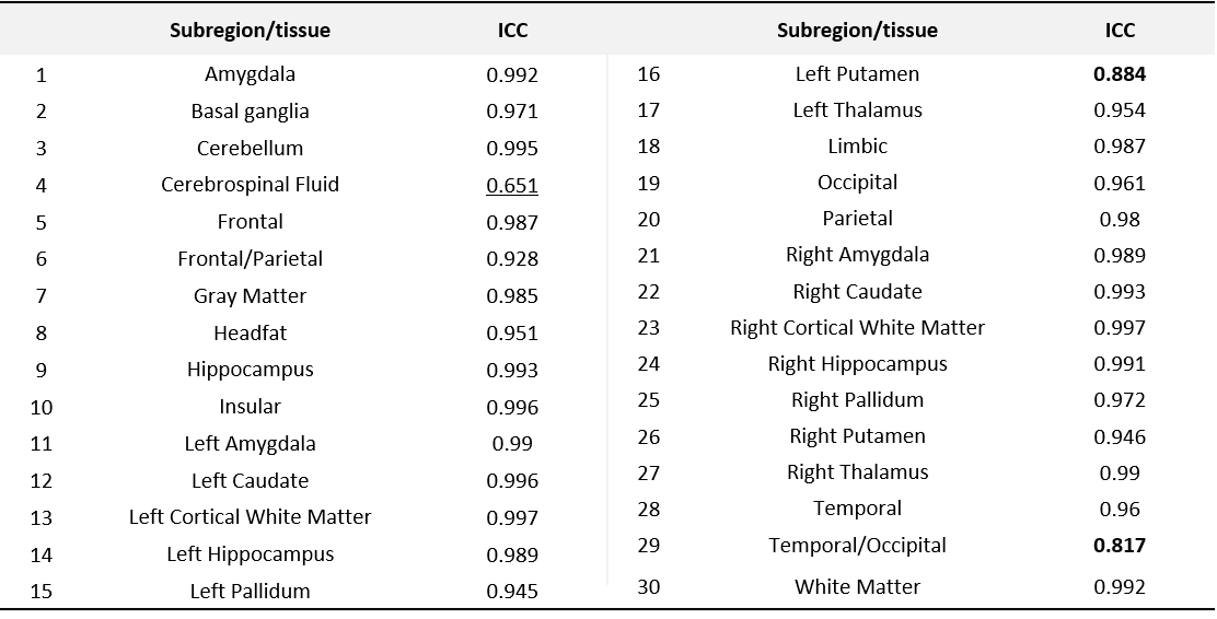
Figure 1 presents the sequences in the GS protocol. Sequence-specific LUTs were constructed by recording relative signal-to-noise ratio (rSNR) values and acquisition durations from the vendor UI, as described in prior work2. These LUTs were consulted to derive optimal acquisition parameters for each sequence, and the Fastest protocol was assembled. 2D convolutional neural networks were trained on publicly available datasets to perform 64x64 patch-wise contrast-specific image-denoising (Figure 2). These datasets were assumed to be noise-free and were corrupted with native noise3,4. An iterative, local-SNR-guided5 process determined the noise scaling factor. The loss function was a weighted combination of L1 loss and a data-consistency term in the Fourier domain. These baseline models were fine-tuned to achieve subject-specific (SS) denoising since MR physics dictates that SNR is subject-dependent. Four experiments were performed to (i) determine the impact on throughput measured via table time, (ii) quantitatively measure image quality, (iii) investigate recovery of image quality using DL, and (iv) test for repeatability across five exams. Five healthy volunteers were imaged utilizing the GS and Fastest protocols. Peak SNR (PSNR), multi-scale SSIM (MS-SSIM), and the variance of the Laplacian6 (var-Lap) were computed. Automated volumetry was performed on T1w data using a tool that leveraged two DL networks which are developments on prior work7. The tool reported volumetric measures of 27 brain anatomies and 3 brain tissues. The mean of RMSEs of all volumetric measures was computed to compare the four methods: GS, Fastest, baseline-denoised Fastest, and SS-denoised Fastest. The intra-class correlation coefficient (ICC) based on the analysis of variance (ANOVA) with repeated measures was calculated to assess the agreement of the volumetric measures amongst the GS, baseline-denoised, and SS-denoised methods. For the remaining contrasts, manual volumetry was performed by four MR-experienced raters on incidental benign white matter hyperintensities on one subject’s data.Results and discussion
The LUT approach adopted in this work is (i) easily scalable if querying the vendor UI can be automated, and (ii) extensible to allow optimizing for different criteria. Shorter acquisition times were the focus of this work. The GS protocol was accelerated from 17:23 (minutes:seconds) to 8:34 (Fastest). From experiment 1, employing this protocol resulted in a 1.94x gain in practical imaging throughput. Figure 3 presents representative slices of data from an arbitrarily chosen subject’s acquisition, for all contrasts, across both protocols. Although we aimed to derive an accelerated protocol without affecting image contrast, we observe a marginal shift in contrast in the Fastest data. The table in Figure 3 presents the median local SNR values. The Fastest data performs comparably for T2 FLAIR, and poorer than GS in the rest. For the contrast-specific image-denoising models in experiment 3, the model achieving the lowest validation loss was chosen in every instance. We adopted a patch-wise approach in this work to avoid biasing the models from learning any brain anatomies. However, this results in an increase in inference duration, proportional to the number of patches per input slice. It can be observed from Figure 4 that baseline-denoising yielded the largest improvements in PSNR, MS-SSIM, and var-Lap for the T2 contrast. The var-Lap metric is on an arbitrary scale and hence precludes comparing methods without controlling for the testing datasets. For SS-denoising, the largest gains were similarly observed on the T2 contrast, followed by T2 FLAIR. For T1, SS-denoising results in no improvement in PSNR, but modest gains in MS-SSIM accompanied by reduced blurriness. SS-denoising demonstrated improved recovery of image quality and increased the accuracy of T1 volumetry. From experiment 4, for all 30 locations across the four methods, 27 had excellent ICC (>=0.93); 2 had a good ICC (>0.8), and 1 had moderate ICC (=0.651). Figure 5 lists the individual ICC values for each of the 27 brain subregions and the 3 brain tissues.Conclusion
We demonstrated the application of deep learning to perform image-denoising of accelerated acquisitions to improve imaging throughput by 1.94x. Since the protocol constitutes 42.85% and 44.44% of the protocols prescribed by the Alzheimer’s Disease Neuroimaging Initiative (https://adni.loni.usc.edu/) and the European Prevention of Alzheimer’s Disease project (https://ep-ad.org/), respectively, the Fastest protocol could potentially be utilized for accelerated AD imaging.Acknowledgements
No acknowledgement found.References
- Geethanath, S. and Vaughan Jr, J.T., 2019. Accessible magnetic resonance imaging: A review. Journal of Magnetic Resonance Imaging, 49(7), pp.e65-e77.
- Ravi, K.S., Geethanath, S., Quarterman, P., Fung, M. and Vaughan Jr, J.T., 2020. Intelligent Protocolling for Autonomous MRI. ISMRM.
- Geethanath, S., Poojar, P., Ravi, K.S. and Ogbole, G., 2021. MRI denoising using native noise. In Proc Intl Soc Mag Reson Med (Vol. 2405).
- Qian, E., Poojar, P., Vaughan Jr, J.T., Jin, Z. and Geethanath, S., 2022. Tailored magnetic resonance fingerprinting for simultaneous non‐synthetic and quantitative imaging: A repeatability study. Medical Physics, 49(3), pp.1673-1685.
- Golshan, H.M., Hasanzadeh, R.P. and Yousefzadeh, S.C., 2013. An MRI denoising method using image data redundancy and local SNR estimation. Magnetic resonance imaging, 31(7), pp.1206-1217.
- Pech-Pacheco, J.L., Cristóbal, G., Chamorro-Martinez, J. and Fernández-Valdivia, J., 2000, September. Diatom autofocusing in brightfield microscopy: a comparative study. In Proceedings 15th International Conference on Pattern Recognition. ICPR-2000 (Vol. 3, pp. 314-317). IEEE.
- Thomas, N., Perumalla, A., Rao, S., Thangaraj, V., Ravi, K.S., Geethanath, S., Kim, H. and Srinivasan, G., 2020, October. Fully automated end-to-end neuroimaging workflow for mental health screening. In 2020 IEEE 20th International Conference on Bioinformatics and Bioengineering (BIBE) (pp. 642-647). IEEE.
Figures

Figure 1. Protocols and datasets. Sequences comprising the Gold Standard (GS) and Fastest protocols, and their corresponding acquisition durations. Employing the Fastest protocol resulted in a 1.94x gain in practical imaging throughput. The SWI sequence in the GS protocol was substituted by the T2* sequence. The second table lists the contrast-specific publicly available datasets that were used to train the image-denoising models.
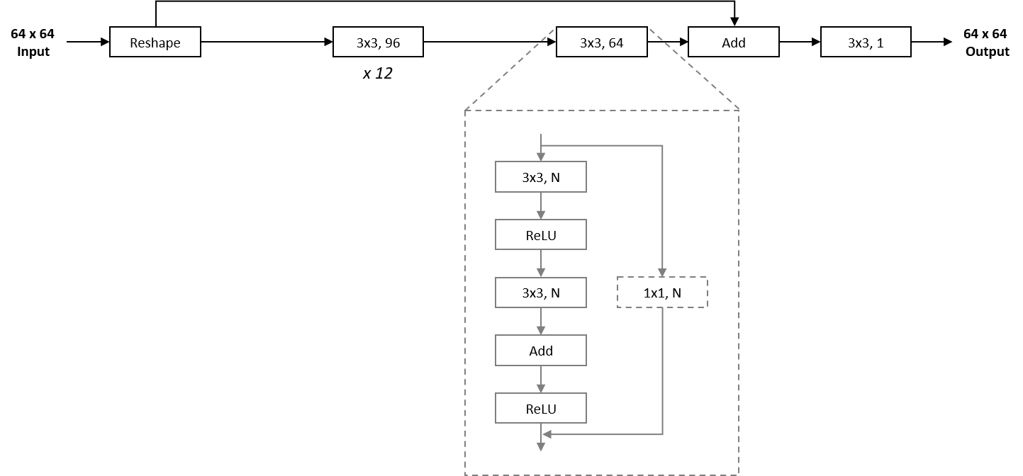
Figure 2. Network architecture of image-denoising models. The overall architecture of the patch-wise approach in this work employed a ResNet-style skip-connection for faster convergence and improved stability. Input data was reshaped as a preprocessing step, and 12 2D convolution layers with 96 filters each were utilized, followed by another layer with 64 filters. Finally, the input data was added to this residual output via an identity skip connection, before being collapsed to a single channel via another 2D convolution layer.
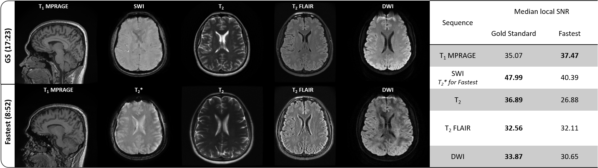
Figure 3. Representative slices and quantative image quality metrics of Gold Standard (GS) and Fastest data. A single representative slice across contrasts from GS and Fastest data of an arbitrarily chosen subject is shown. The corresponding median local SNR values are also presented in the table on the right.

Figure 4. Quantitative performance evaluation of baseline-denoising models. PSNR (dB), MS-SSIM, and the variance of the Laplacian (var-Lap) were measured on the denoised images from the test sets. The improvements in these metrics for each contrast are reported. For var-Lap, lower is better.