4628
Improving Spiral Deblurring with Square Kernels and Low-Pass Preconditioning1Department of Radiology, Mayo Clinic, Rochester, MN, United States
Synopsis
Keywords: Image Reconstruction, Artifacts, spiral imaging, deblurring, off-resonance
Advantages of spiral imaging include fast scan speed and high SNR efficiency. Success implementation of spiral imaging relies on utilization of efficient deblurring methods. The goal of this work is to improve the performance of a previous deblurring method, using square kernels and low-pass preconditioning. Data from phantom and volunteers demonstrate that artifacts can be reduced while computational demand is also reduced by the proposed kernels.
Introduction
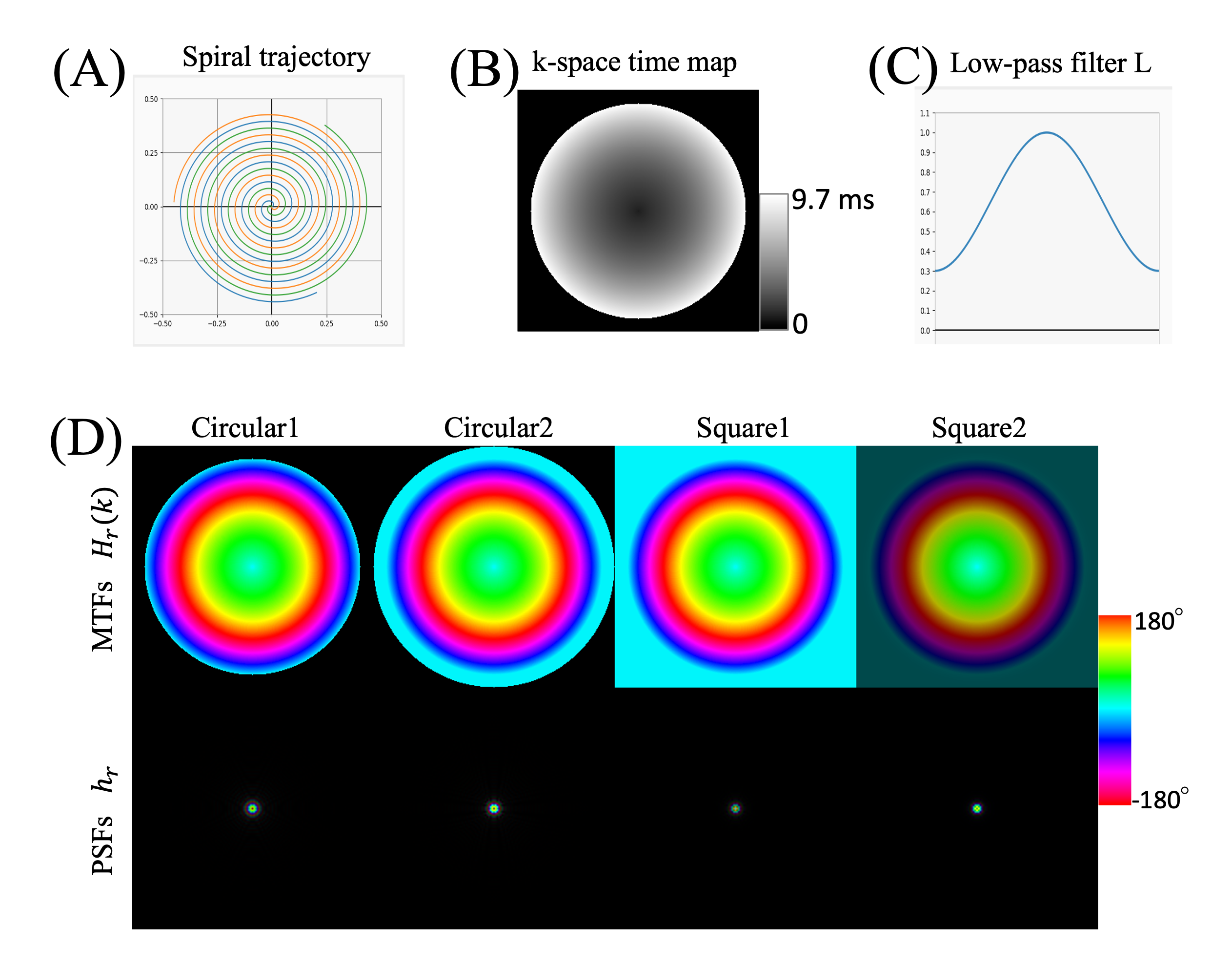
Spiral imaging has been implemented for many applications, including high resolution brain imaging1, for its favorable characteristics such as fast imaging and high SNR efficiency. Since both off-resonance and chemical shift cause blurring in spiral images, deblurring plays a critical role in spiral imaging. A method was proposed2 to jointly deblur water and fat using blurring/deblurring kernels in the image space. The quality and efficiency of the deblurring largely depends on the properties of the kernels. In this study, we propose to use modified kernels as well as low-pass preconditioning3 to improve the performance of the deblurring.Theory
The blurring process can be described as$$$Bf = g$$$, (1)
where g represents the blurred TE images and f represents the underlying "true" water and fat images, and the matrix B models the effects of off-resonance blurring. An estimate of f can be obtained by iteratively solving
$$$B^HBf = B^Hg$$$, (2)
using a conjugate gradient method4, where BH is the conjugate transpose of B. The processes B and BH are computed by implementing spatially-varying image-space convolution using blurring and deblurring kernels, respectively2. As shown in Fig. 1, the modulation transfer function (MTF) of the blurring kernel, $$$Η_r(k)$$$, has a magnitude of one and a phase proportional to the product of the time map of the spiral trajectory and the off-resonance $$$Δ f_0(r)$$$. The inverse Fourier transform of $$$Η_r(k)$$$ gives a spatially-varying point spread function (PSF) $$$h_r$$$. Since the PSFs are much more compact than MTFs (Fig.1 D), computing the blurring with spatially-varying convolutions is fairly efficient.
Applying a low-pass filter L to Eq.(1), we have.
$$$LBf = Lg$$$. (3)
This amounts to preconditioning. An estimate of the same underlying f can be obtained by iteratively solving3
$$$(LB)^H(LB)f = (LB)^HLg,$$$ (4)
in which Lg is the low-pass filtered version of the TE images. The kernels corresponding to LB are the low-pass filtered version of kernels corresponding to B.
Methods
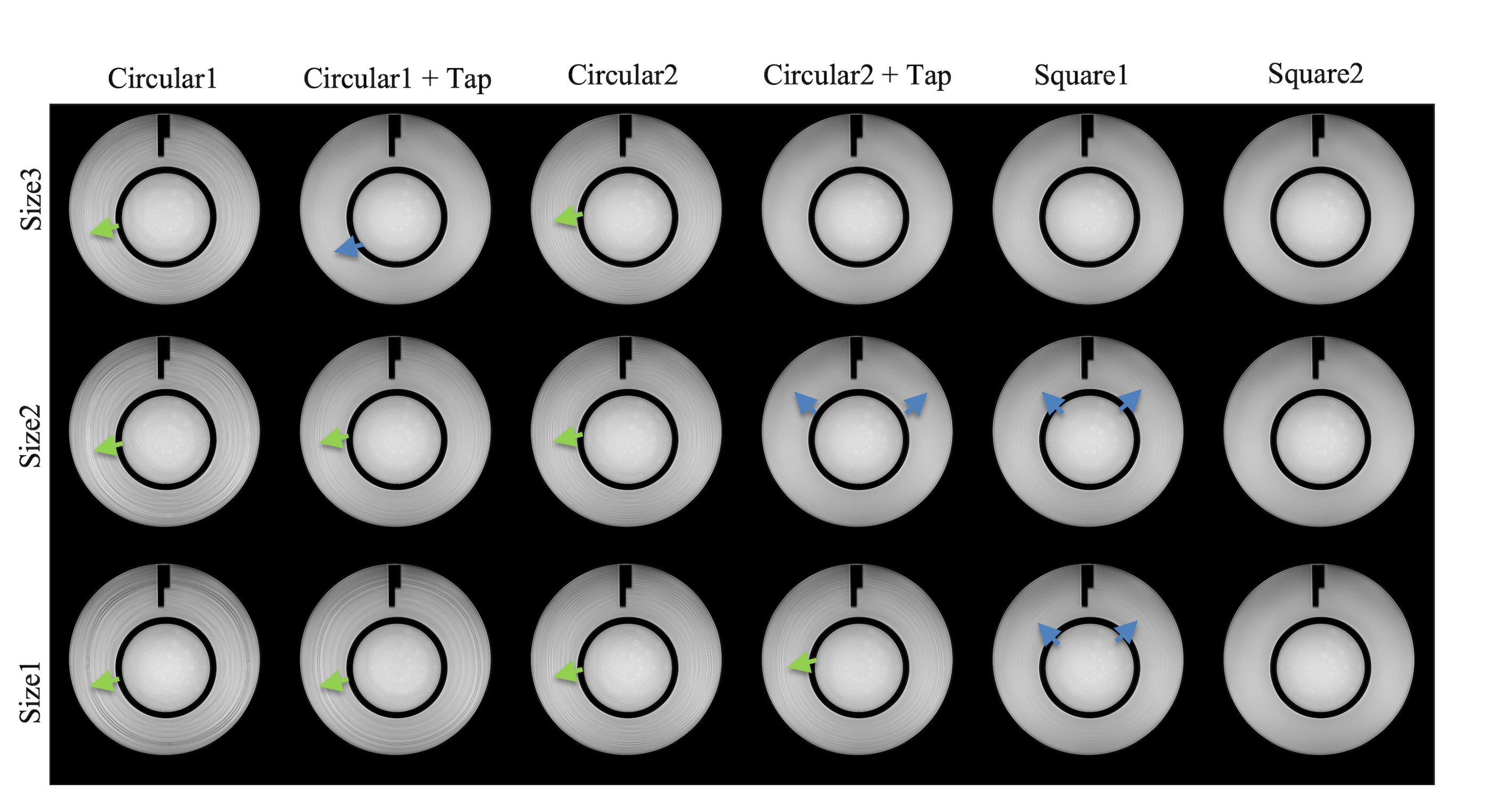
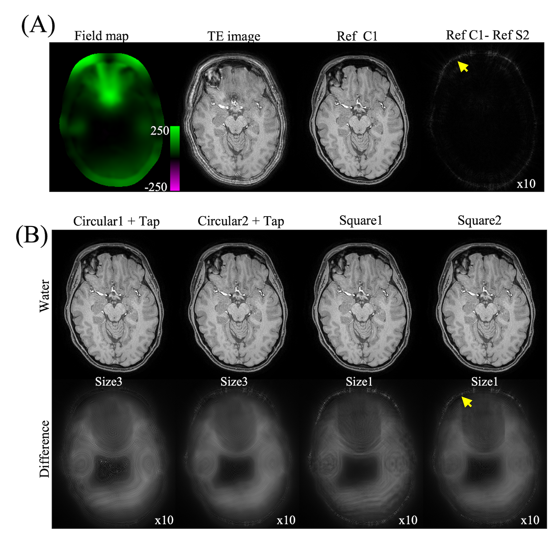
The diameter of the acquired spiral k-space is $$$2/\sqrt{\pi} \approx 1.13$$$ times of width of the Cartesian k-space to cover the same total area5. The k-space matrix width is also increased by 25% over the prescribed FOV/resolution ratio, for convenience in gridding the collected data. In this study, we compare four kinds of kernels (Fig. 1 (D)). In the previous work the magnitude of the k-space blurring MTF was set to zero outside of the collected region2. This is the first type of kernels (circluar1). In the second type, the unit magnitude and the maximum accumulated phase are extended to a larger circle tangent to the border (circular2). This coverage is further extended to the comers of the k-space for the third type of kernels (square1). Using the low-pass preconditioned deblurring (Eqs (3-4)), a low-pass filter L as shown in Fig.1 (C) is applied to square1, forming the fourth type of kernels (square2).The energy was computed for various kernel sizes and normalized by the total energy of the full-size kernels to estimate the compactness of different kernels. Water-fat separation and deblurring were tested on phantom and volunteer brain data that were collected at two TEs with ΔTE = 1.15 ms on a 3 Tesla Philips scanner (Philips Healthcare, Best, The Netherlands). The field maps of $$$Δ f_0(r)$$$ were obtained from separate low-resolution scans. The widths of the kernels were $$$CΔ f_0(r)τ+2b+1$$$, where τ is the sampling time. In this study, C is 27.6 and b is set to 2 (size1), 3 (size2) and 5 (size3) respectively. The results were compared to the reference data using full-size kernels to obtain normalized root mean square error (NRMSE). The spiral trajectories, one set of the reference images and $$$Δ f_0(r)$$$ from the experiment were used to synthesize k-space data by discrete Fourier transform. Noise was also synthesized for the same trajectories to evaluate the SNR2.
Results and Discussion
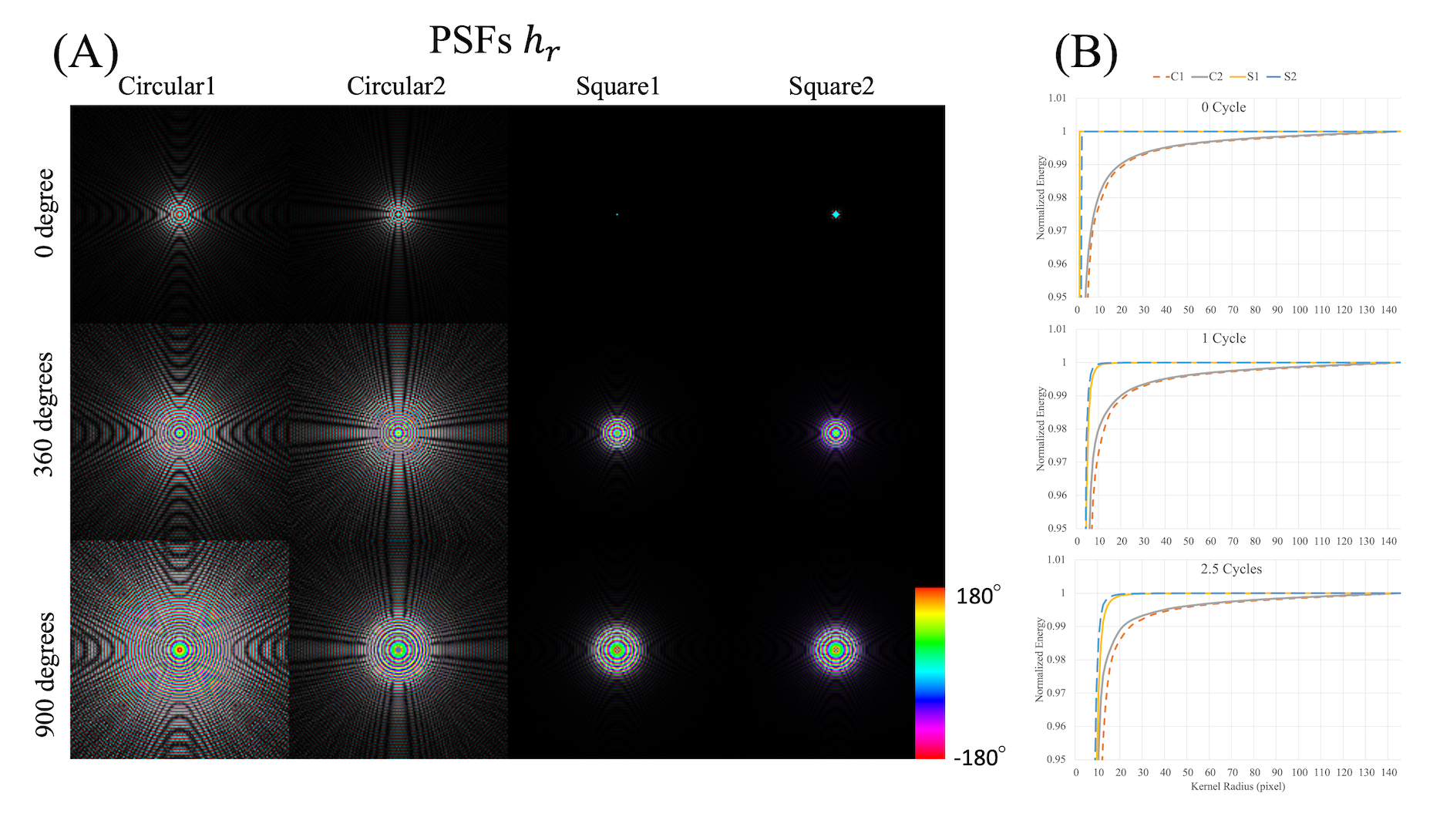
The square kernels are much more compact than the circular kernels as shown in Fig.2. Square2 kernels are slightly wider than square1 kernels with low values of $$$Δ f_0$$$. They become slightly more compact when $$$Δ f_0$$$ reaches 23 Hz (τ = 9.7 ms), corresponding to maximum accumulated phase of 80 degrees (0.22 cycle). The influences of kernel compactness can be seen with phantom images in Fig. 3. The circular kernels produce more artifacts on flat areas of the phantom than the square kernels. Tapering the circular kernels at the edges in the image space can mitigate the artifacts, while the square kernels produce similar or less artifacts without tapering. Square2 kernels demonstrate the best performance for all three kernel sizes for mitigation of artifacts.Some volunteer results are shown in Fig.4 and Table1. The square kernels of size1 yield images with similar visual appearance and better NRMSE compared to the tapered circular kernels of size3, with a reduction of the computational cost by 44%. The SNRs using circluar2, square1 and square2 are comparable, which are 6-9% higher than the SNR using circular1 kernels.
Conclusions
The sizes of the blurring kernels and thus the computational cost can be reduced by more compact square kernels instead of the previous circular ones. Using low-pass preconditioning may further enhance the performance.Acknowledgements
This work was funded by Philips Healthcare.
References
1. Ooi MB, Li Z, Robison RK, Wang D, Anderson AG, Zwart NR, et al. Spiral T1 Spin-Echo for Routine Postcontrast Brain MRI Exams: A Multicenter Multireader Clinical Evaluation. Am J Neuroradiol. 2020 Feb;41(2):238–45.
2. Wang D, Zwart NR, Pipe JG. Joint water-fat separation and deblurring for spiral imaging. Magn Reson Med. 2018;79:3218-3228.
3. Wang D, Robison RK, Li Z, Pipe JG. High SNR rapid T1-weighted MPRAGE using spiral imaging with long readouts and improved deblurring. Magn Reson Med. 2022;1-13. doi: 10.1002/mrm.29492.
4. Shewchuk JR. An introduction to the conjugate gradient method without the agonizing pain; 1994. Available at: https:// www.cs.cmu.edu/~quake-papers/painless-conjugate-gradient. pdf. [Accessed March 14, 2017].
5. Van Gelderen P. Comparing true resolution in square versus circular k-space sampling. Proceedings of the 6th Annual Meeting of ISMRM, Sydney, Australia, 1998. p 424.
Figures
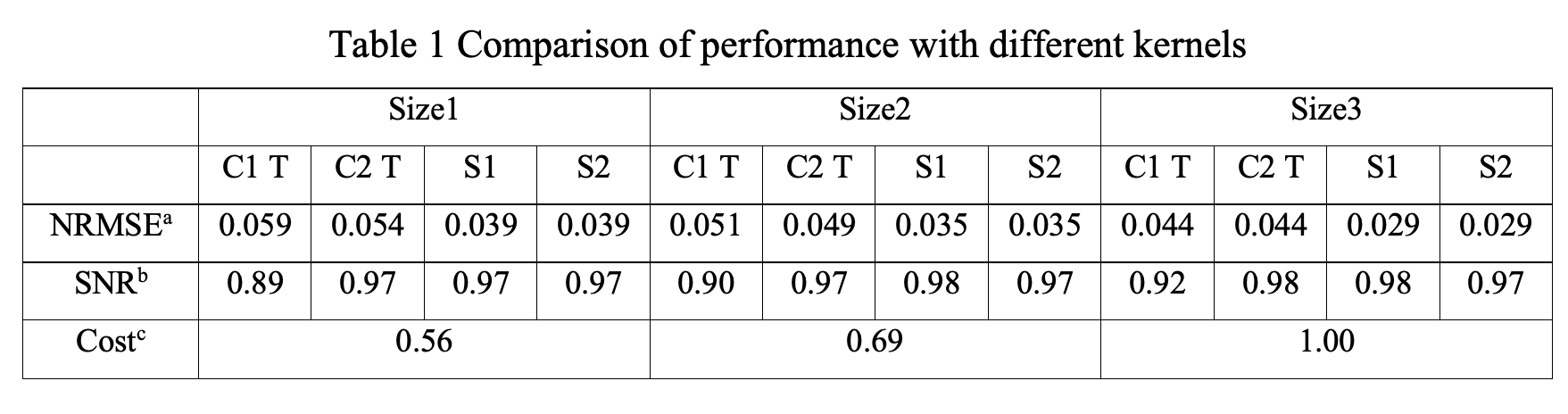
The estimation is based on the slice of volunteer data shown in Fig. 4. The in-plane resolution is 1.0 x 1.0 mm2. The sampling time τ is 9.7 ms. C1, circular1; C2, circular2; S1, square1; S2, square2; T, kernel tapering at image space; NRMSE, normalized root mean square error.
a RMSE was calculated with respect to the reference image of the specific kernel type and then normalized by the mean of the image magnitude.
b This is SNR relative to the SNR of the average of two TE images.
c Relative computational cost.