4622
Water removal in MR spectroscopic imaging with Casorati Singular Value Decomposition
Amirmohammad Shamaei1, Jana Starcukova1, Jedrek Burakiewicz 2, and Zenon Starcuk 1
1Institute of Scientific Instruments of the Czech Academy of Sciences Research institute in Brno, Brno, Czech Republic, 2Tesla Dynamic Coils, Zaltbommel, Netherlands
1Institute of Scientific Instruments of the Czech Academy of Sciences Research institute in Brno, Brno, Czech Republic, 2Tesla Dynamic Coils, Zaltbommel, Netherlands
Synopsis
Keywords: Sparse & Low-Rank Models, Data Processing, Singular value decomposition, MR spectroscopic imaging, Water removal
Removing residual water from the MRSI datasets using the SVD-based algorithms is computationally demanding. We present a novel algorithm to reduce the computing time required for water removal in MRSI data. Our proposed method exploits low-rank structures that exist in MRSI data. It arranges the MRSI data in the Casorati matrix form, applies singular value decomposition, and removes residual water from the most prominent left-singular vectors. We compared our proposed method with the HLSVDPRO method, and we achieved 20x acceleration while improving effectiveness. Our proposed method is publicly available as a pip-installable Python tool.INTRODUCTION
Singular value decomposition (SVD) is typically used as the foundation of post-processing residual water removal procedures for in vivo MR spectroscopic imaging (MRSI) data 1,2.SVD-based approaches model and remove the water signal on the premise that MRSI signals in the time domain can be characterized by a model consisting of a small number of exponentially damped sinusoids 1,2. Removing residual water from the MRSI datasets using L2 regularization 3, tensor-based 4, and low-rank reconstruction techniques 5 has also been suggested.
The calculation of the singular value decomposition (SVD) is computationally demanding. Moreover, in an MRSI dataset the SVD of a Hankel matrix should be calculated for each signal. Thus, water removal is one of the computational bottlenecks in the processing of high-resolution MRSI data.
Our objective is to reduce the computing time required for water removal in MRSI data.
THEORY
Spatiotemporal Partial Separability$$$D_0$$$ is an MRSI data matrix with an assumption that all signals in $$$D_0$$$ lie in a low-dimensional subspace embedded in a higher-dimensional space. The $$$D_0$$$ can be expressed as partially separable to the $$$L$$$-th order:
$$D_0\left(k,t\right)=\ \sum_{l=1}^{L}{c_l\left(k\right)\psi_l\left(t\right)}, (1) $$
where $$$c\left(k\right)$$$ and $$$ \psi\left(t\right) $$$ can be viewed as the common basis among signals and the temporal basis for $$$D_0\left(k,t\right)$$$, respectively.
A Casorati matrix can be constructed from $$$D_0\left(k,t\right)$$$ and has at most rank L.
$$C_0\ =\ \left[\begin{matrix}\begin{matrix}D_0\left({k}_1,t_1\right)&D_0\left({k}_2,t_1\right)\\D_0\left({k}_1,t_2\right)&D_0\left({k}_2,t_2\right)\\\end{matrix}&\begin{matrix}\cdots&D_0\left({k}_M,t_1\right)\\\ldots&D_0\left({k}_M,t_2\right)\\\end{matrix}\\\begin{matrix}&\ldots\\D_0\left({k}_1,t_N\right)&D_0\left({k}_2,t_N\right)\\\end{matrix}&\begin{matrix}&\\\ldots&D_0\left(k_M,t_N\right)\\\end{matrix}\\\end{matrix}\right], (2)$$
where $$$N$$$ and $$$M$$$ are the number of time points and the number of voxels, respectively.
Singular Value Decomposition
The SVD is a factorization of a complex $$$n \times m$$$ matrix $$$C$$$ in the following form:
$$C=U \Sigma V^\ast , (3)$$ where $$$U$$$ is an $$$n \times m$$$ complex unitary matrix, $$$\Sigma$$$ is an $$$n \times m$$$ rectangular diagonal real matrix with non-negative real numbers on the diagonal in descending order, $$$V$$$ is an $$$n \times m$$$ complex unitary matrix, and $$$\ast$$$ is the conjugate transpose.
METHODS
Given a measured MRSI data matrix $$$D$$$, the proposed algorithm is described in the following steps:Step 1. For D, construct Casorati matrix C according to Eq. 2.
Step 2. Compute the SVD of the Casorati matrix according to Eq. 3 to obtain $$$U$$$, $$$\Sigma$$$, and $$$V$$$.
Step 3. Determine the rank ($$$r$$$) of $$$C$$$. In this work, the optimal singular value hard thresholding 6 method was utilized for automatically estimating the rank of matrix $$$C$$$.
Step 4. Apply HLSVDPRO 2 on each of the first $$$r$$$ columns of $$$U$$$, and remove the residual water signal. Store water-removed signals in the corresponding columns of matrix $$$U$$$.
Step 5. Construct the water-removed matrix $$$\hat{C}$$$ using Eq. 3.
In the proposed algorithm, due to the low rank of $$$C$$$, we apply the HLSVDPRO algorithm only on the few columns of $$$U$$$ instead of each signal in dataset $$$D$$$ $$$(r\ \ll\ M)$$$.
We have developed the CSVD algorithm in Python programming language and released it as an open-source pip-installable Python tool (https://pypi.org/project/CSVD/).
In vivo 1H MRSI data
The LTE‐WS‐MRSI is publicly accessible MRSI data 3 from a healthy volunteer acquired on a Philips Achieva 3T scanner (field of view = 230 × 172.5 mm2; slice matrix = 32 × 24; slice thickness = 15 mm; echo time (TE) = 140 ms; repetition time (TR) = 3.2 s; sample bandwidth = 2000 Hz; sample points = 512; a WET scheme for water suppression; a 32‐channel head coil).
Implementation details
The HLSVDPRO and CSVD methods for removing residual water signals from the LTE‐WS‐MRSI datasets were compared. We set the model order (number of components) and the water removal range to 30 and 4.7 ± 0.6 ppm in HLSVDPRO and CSVD algorithms (Step 4).
RESULTS & DISCUSSION
The rank of the constructed Casorati matrix was set to 30 by the optimal singular value hard thresholding algorithm, which was much lower than the original dimensionality of data (32 × 24 = 768). Figure 1 illustrates the structure of the Casorati matrix and the first 50 singular values. Figure 2 shows the first 3 spectra (columns) of matrix U. Figure 3 illustrates the results of HLSVDPRO and CSVD methods on the LTE‐WS‐MRSI dataset. Original spectra from selected voxels were shown along with the corresponding water-removed spectra. While Figure 3c shows that the CSVD and the HLSVDPRO work well, Figure 3a shows that the HLSVDPRO cannot adequately remove the residual water signal. Figures 3b and 3d show that removing water using the HLSVDPRO results in baseline distortion. Processing time for HLSVD and CSVD methods for the LTE‐WS‐MRSI dataset were 24.8 and 1.4 seconds, respectively.CONCLUSION
The results from in vivo MRSI data demonstrate that the CSVD method can adequately remove residual water signals in a significantly shorter amount of time than the HLSVD. The CSVD method effectively removes baseline distortions caused by the large water peak. The proposed method may also be used to remove contamination from peri-cranial lipid resonances. One limitation of this work is that if the residual water signal is not well characterized by the model (Lorentzian line shape) in the HLSVDPRO algorithm (Step 4), the CSVD may not yield satisfactory results. One of the possible remedies would be to fit a Voigt line instead.Acknowledgements
This project has received funding from the European Union's Horizon 2020 research and innovation program under the Marie Skłodowska-Curie grant agreement No 813120.References
1. Cabanes E, Fur Y Le, Simond G, Cozzone PJ. Optimization of Residual Water Signal Removal by HLSVD on Simulated Short Echo Time Proton MR Spectra of the Human Brain. 2001;125:116-125. doi:10.1006/jmre.2001.23182. Laudadio T, Mastronardi N, Vanhamme L, Van Hecke P, Van Huffel S. Improved Lanczos algorithms for blackbox MRS data quantitation. J Magn Reson. 2002;157(2):292-297. doi:10.1006/jmre.2002.2593
3. Lin L, Považan M, Berrington A, Chen Z, Barker PB. Water removal in MR spectroscopic imaging with L2 regularization. Magn Reson Med. 2019;82(4):1278-1287. doi:10.1002/mrm.27824
4. Nagaraja BH, Debals O, Sima DM, Himmelreich U, De Lathauwer L, Van Huffel S. Tensor-based method for residual water suppression in 1 H magnetic resonance spectroscopic imaging. IEEE Trans Biomed Eng. 2019;66(2):584-594. doi:10.1109/TBME.2018.2850911
5. Bhattacharya I, Jacob M. Compartmentalized Low-Rank Recovery for High-Resolution Lipid Unsuppressed MRSI. Magn Reson Med. 2017;78:1267-1280. doi:10.1002/mrm.26537
6. Gavish M, Donoho DL. The Optimal Hard Threshold for Singular Values is 4/sqrt(3). IEEE Trans Inf Theory. 2013;60(8):5040-5053. doi:10.1109/TIT.2014.2323359
Figures
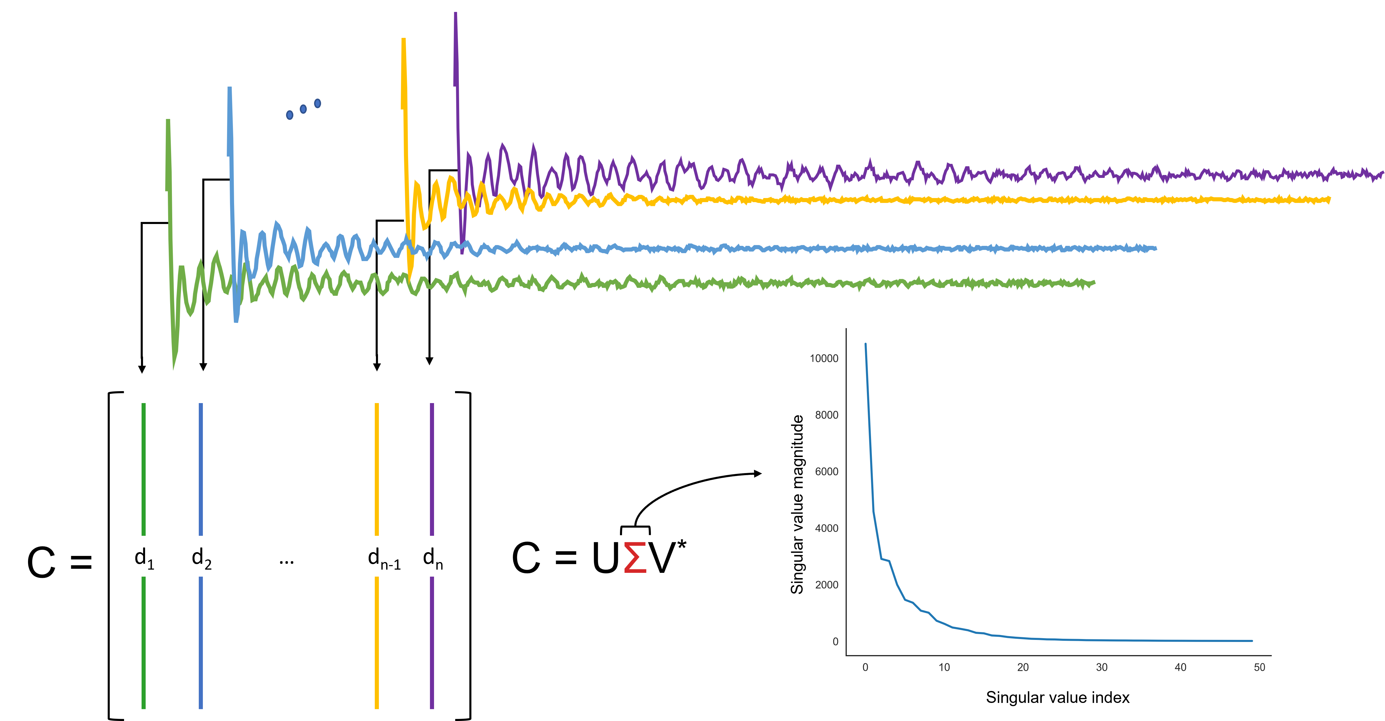
Figure 1. Visualization of the structure of Casorati matrix and the first 50 singular values.
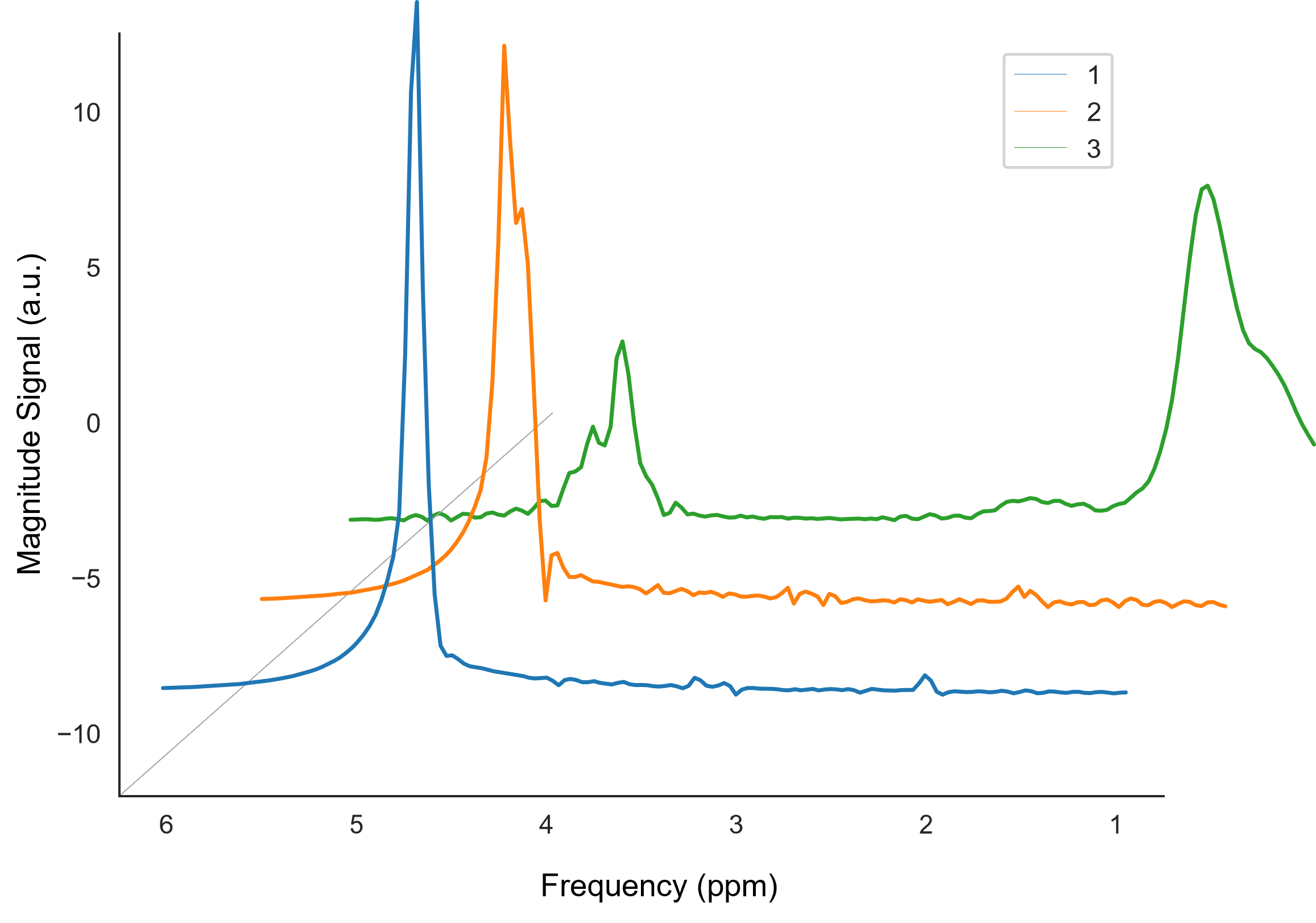
Figure 2. Illustration of the first 3 spectra (columns) of the left
singular vectors.
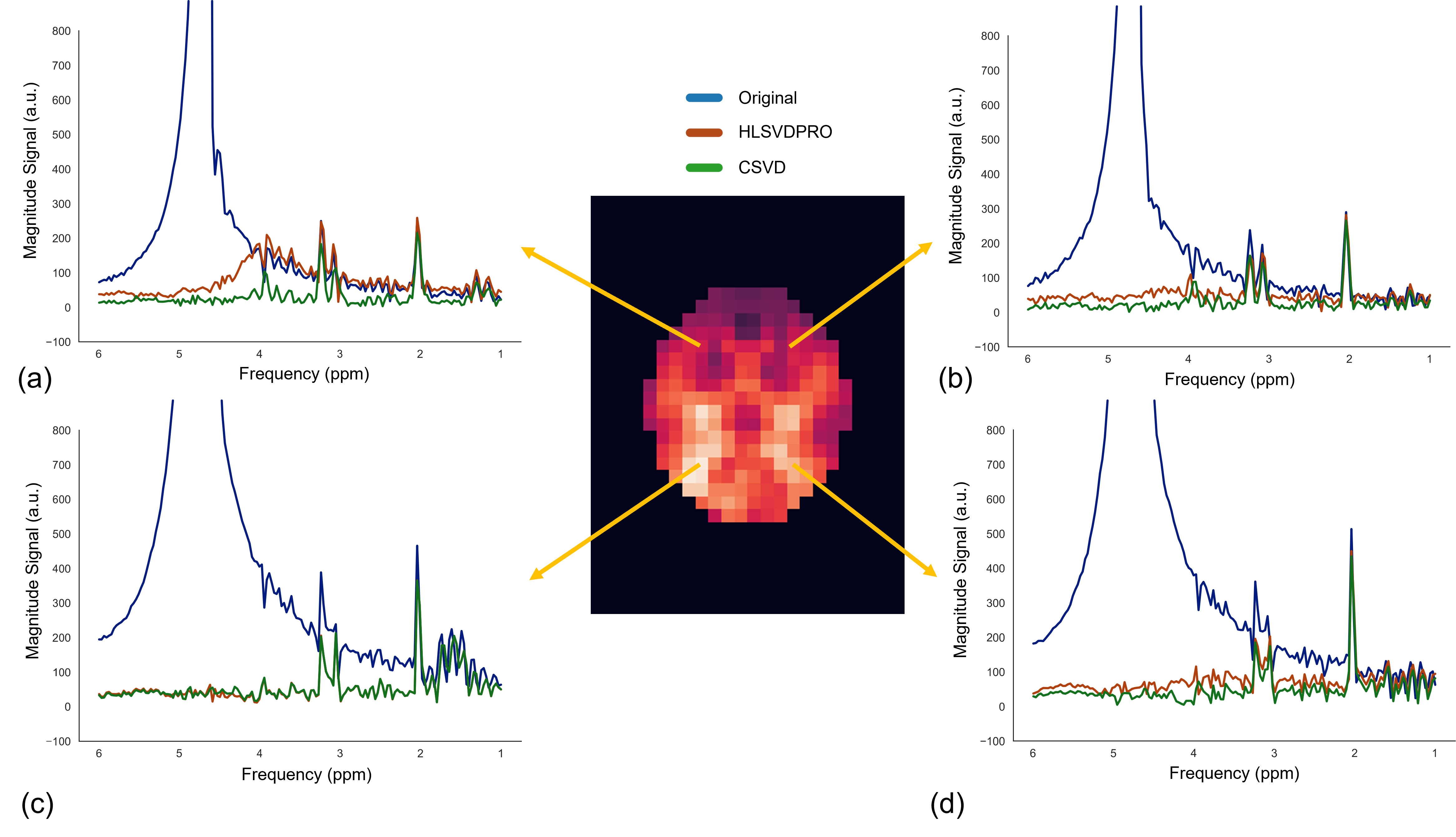
Figure 3. Comparison of HLSVDPRO and CSVD methods for the LTE‐WS‐MRSI dataset. (a-d) Representative original spectra from the selected voxels along with the corresponding water-removed spectra. . (a-d) Representative original spectra from the selected voxels along with the corresponding water-removed spectra.
DOI: https://doi.org/10.58530/2023/4622