4619
Time-Resolved MRI Kinesiology: Reconstructing force and velocity during active loading1Department of Radiotherapy, Computational Imaging Group for MR Diagnostics and Therapy, UMC Utrecht, Utrecht, Netherlands
Synopsis
Keywords: Signal Modeling, MSK, Time-Resolved, Velocity, Force, Motion
Force and velocity are two important quantities for studying muscles, but retrieving these quantities using MRI is challenging. Spectro-Dynamic MRI allows the characterization of dynamical systems at a high spatial and temporal resolution directly from k-space data. Using an iterative reconstruction algorithm, we can reconstruct time-resolved MR images, time-resolved motion fields, mechanical parameters, and an activation force, at a temporal resolution of 11 ms. As a proof-of-principle, MR data was acquired with a motion phantom moving like an actively driven linear elastic system. All dynamic variables could be reconstructed accurately. This method could become useful for studying muscles under dynamic loads.
Introduction
Kinesiology studies the dynamics of the human body, for example by analyzing the force and velocity within muscle tissue. These two quantities are important to understand the mechanisms of skeletal muscle contraction or the pathophysiology of muscular diseases1. Dynamic MRI can be a useful tool to acquire this information2, but acquiring 3D dynamic data at high temporal resolutions is challenging. There is currently no unified and comprehensive MRI framework for full dynamic characterization of a system. We have proposed Spectro-Dynamic MRI3 as a method to acquire time-resolved dynamic information at a high spatio-temporal resolution directly from k-space data. This goes beyond capturing moving images, by coupling the dynamic k-space measurements to the underlying motion and physics. Here we present an extended Spectro-Dynamic MRI framework which is able to reconstruct: (1) time-resolved images, (2) time-resolved motion fields, (3) mechanical parameters, and (4) an activation force. This framework is applied to experimental data from a dynamical phantom as a proof-of-concept, capturing its dynamics with four degrees of freedom at a temporal resolution of 11 ms.Theory
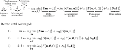
Our reconstruction solves an optimization problem with four terms (Fig. 1). The first term enforces consistency between the undersampled measured data $$$\mathbf{d}$$$ and the full spatio-temporal k-space data $$$\mathbf{m}$$$, where $$$E$$$ contains the sampling pattern. The second term is the measurement model $$$G(\mathbf{m},\mathbf{u})$$$, which relates the k-space data $$$\mathbf{m}$$$ to the displacement fields $$$\mathbf{u}$$$ using a partial differential equation similar to the optical flow model3. Finite differences are used to evaluate the temporal derivatives in this model. The third term, $$$F(\mathbf{u},\boldsymbol{\theta},\mathbf{f})$$$, is the dynamical model. This model describes the dynamics of the system under investigation, and constrains the displacement vector field $$$\mathbf{u}$$$ using a set of mechanical parameters $$$\boldsymbol{\theta}$$$ and forcing term $$$\mathbf{f}$$$. Thus, the measurement model links the k-space data to the motion fields, while the dynamical model provides the connection to the underlying physics. Finally, a regularization promoting temporal smoothness is applied to $$$\mathbf{f}$$$ using the second-order temporal finite difference operator $$$D_{tt}$$$. This optimization problem is solved for $$$\mathbf{m}$$$, $$$\mathbf{u}$$$, $$$\boldsymbol{\theta}$$$, and $$$\mathbf{f}$$$. Since the minimization is linear for each parameter individually, the optimization problem can be solved by alternating solutions of a series of linear least-squares problems (Fig. 1).Methods
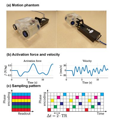
Experimental data was acquired using the Quasar MRI4D Motion Phantom (Modus Medical Devices Inc.). This dynamical phantom (Fig. 2a) consists of one stationary compartment filled with water, one stationary gel-filled cylinder, and one moving compartment with two gel-filled tubes (TO5, Eurospin II test system). An actively driven linear elastic system with stiffness coefficient $$$k$$$ and activation force $$$f(t)$$$, both normalized by the mass, functioned as the dynamical model:$$\ddot{u}(t)+ku(t)=f(t)\tag{1}$$
This frequently used model allows for a large variety of dynamics through different choices for $$$\mathbf{f}$$$. The numerical solution $$$u(t)$$$ of Eq. 1, given the activation as shown in Fig. 2b and a (mass-normalized) stiffness coefficient of 30 N/m/kg, was given as the position setpoint to the phantom.
The experiments were performed using a 1.5T MRI scanner (Ingenia, Philips Healthcare) with a spoiled gradient echo sequence (TR/TE=5.5/2.2 ms, FA=5$$$^\circ$$$). The data was acquired in the coronal plane on a Cartesian grid (FOV=320mm$$$\times$$$320mm, matrix size=64$$$\times$$$64), which was repeated 38 times (Tacq=13.4 s). The k-space was acquired in an interleaved pattern (Fig. 2c) where every two successive readouts were grouped together to better distribute high- and low-frequency data over time.
The lsqr function from Matlab (The MathWorks Inc.) was used to alternatingly solve the linear least squares problems shown in Fig. 1. The displacement vector field was parameterized using four degrees of freedom: the $$$x$$$- and $$$y$$$-displacements for the moving tubes, and those of the stationary objects3.
Results
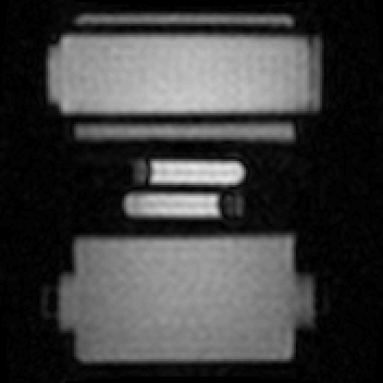
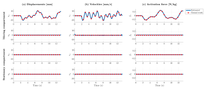
The reconstructed time-resolved images can be seen in Fig. 3, while the estimated displacements and forcing term are shown in Fig. 4. Note that all displacement, velocity and activation force components are accurately reconstructed, including the stationary ones. The estimated mass-normalized stiffness coefficient was 29.3 N/m/kg, very close to the ground truth value of 30 N/m/kg.Discussion
In this proof-of-concept study, all kinematic parameters of the system, meaning the displacements, activation force, and stiffness coefficient could be accurately reconstructed. In addition, time-resolved images could be reconstructed showing the moving phantom at a high temporal resolution of 11 ms, without assuming periodic motion.The in vivo application of our method in 3D requires a model for the dynamical properties of biological tissues. Many constitutive relations for soft tissues exist that are derived from experimental data4. Alternatively, data-driven discovery of dynamical systems5–7 can also be used to generate these models from measured data. Integrating these models in our framework will be the topic of future research. In addition, a low-rank or sparse regularization8,9 on the time-resolved images or displacements fields could be added to deal with the increased undersampling in 3D.
Conclusion
A new reconstruction framework for Spectro-Dynamic MRI has been proposed, which jointly reconstructs time-resolved images, displacement fields, dynamical parameters, and an activation force. The accuracy of this method has been shown using a dynamic phantom as a proof-of-concept. Eventually this method can provide important insights about the dynamic functioning of organs such as muscles.Acknowledgements
We would like to thank Tristan van Leeuwen and David Heesterbeek for fruitful discussions. This work has been financed by NWO, grant number 18897.References
1. Alcazar J, Csapo R, Ara I, Alegre LM. On the Shape of the Force-Velocity Relationship in Skeletal Muscles: The Linear, the Hyperbolic, and the Double-Hyperbolic. Front Physiol. 2019;10. doi:10.3389/fphys.2019.00769
2. Shapiro LM, Gold GE. MRI of weight bearing and movement. Osteoarthritis Cartilage. 2012;20(2):69-78. doi:10.1016/j.joca.2011.11.003
3. van Riel MHC, Huttinga NRF, Sbrizzi A. Spectro-Dynamic MRI: Characterizing Mechanical Systems on a Millisecond Scale. IEEE Access. 2022;10:271-285. doi:10.1109/ACCESS.2021.3138631
4. Chagnon G, Rebouah M, Favier D. Hyperelastic Energy Densities for Soft Biological Tissues: A Review. J Elast. 2015;120(2):129-160. doi:10.1007/s10659-014-9508-z
5. Daniels BC, Nemenman I. Automated adaptive inference of phenomenological dynamical models. Nat Commun. 2015;6:1-8. doi:10.1038/ncomms9133
6. Brunton SL, Proctor JL, Kutz JN, Bialek W. Discovering governing equations from data by sparse identification of nonlinear dynamical systems. Proceedings of the National Academy of Sciences. 2016;113(15):3932-3937. doi:10.1073/pnas.1517384113
7. Rudy SH, Kutz JN, Brunton SL. Deep learning of dynamics and signal-noise decomposition with time-stepping constraints. J Comput Phys. 2019;396:483-506. doi:10.1016/j.jcp.2019.06.056
8. Otazo R, Candès E, Sodickson DK. Low-rank plus sparse matrix decomposition for accelerated dynamic MRI with separation of background and dynamic components. Magn Reson Med. 2015;73(3):1125-1136. doi:10.1002/mrm.25240
9. Huttinga NRF, Bruijnen T, van den Berg CAT, Sbrizzi A. Non-rigid 3D motion estimation at high temporal resolution from prospectively undersampled k-space data using low-rank MR-MOTUS. Magn Reson Med. Published online 2020:1-18. doi:10.1002/mrm.28562
Figures

Figure 1: The extended Spectro-Dynamic MRI framework. The reconstruction minimizes the sum of four terms: a data consistency term, the measurement model, the dynamical model, and a regularization of the forcing term. The relative weighting of these terms is determined by the regularization parameters $$$\lambda_\text{M}$$$, $$$\lambda_\text{D}$$$, and $$$\lambda_\text{R}$$$. The minimization can be split in three independent linear least-squares problems, which are alternatingly solved until convergence.

Figure 2: (a) The motion phantom used during the experiments. (b) The (mass-normalized) activation force used during the experiment, and the resulting velocity as simulated by numerically solving the underlying differential equation (Eq. 1). (c) The sampling pattern used during the experiment. A Cartesian sampling pattern was used, where each phase encode line is depicted using a single color. Every two successive readouts are grouped into a single dynamic snapshot, resulting in an effective $$$\Delta t$$$ of 2 TRs (11 ms).

Figure 3: Estimated time-resolved image at a temporal resolution of 11 ms (2 TRs). These images are obtained by taking the spatial Fourier transform of the estimated fully sampled k-space data. Note that the GIF is displayed at a lower temporal resolution (6 Hz) to limit the file size.

Figure 4: Estimated displacements (a), velocities (b) and mass-normalized activation force (c) for the moving and stationary compartments, in both orthogonal directions. The ground truth value is given by the thin red line and red dots.