4612
PINN with Divergence-Free Vector Potential for Velocity Fields Denoising in 4D flow MRI1Biomedical Imaging Center, Pontificia Universidad Catolica de Chile, Santiago, Chile, 2Department of Electrical Engineering, Pontificia Universidad Catolica de Chile, Santiago, Chile, 3Millennium Institute for Intelligent Healthcare Engineering, iHEALTH, Santiago, Chile, 4Department of Mechanical Engineering, Universidad Técnica Federico Santa Maria, Santiago, Chile, 5School of Biomedical Engineering, Universidad de Valparaíso, Valparaíso, Chile, 6School of Electrical Engineering, Pontificia Universidad Católica de Valparaiso, Valparaíso, Chile, 7Institute for Biological and Medical Engineering, Pontificia Universidad Católica de Chile, Santiago, Chile, 8Department of Radiology, School of Medicine, Pontificia Universidad Católica de Chile, Santiago, Chile
Synopsis
Keywords: Data Processing, Machine Learning/Artificial Intelligence
4D flow MRI suffers from different sources of noise and aliasing artifacts. Recent denoising techniques are time-consuming or dependent of parameter estimation. We developed a physics informed neural network with divergence-free vector potential as a non-parametric denoising technique for 4D flow MRI. Results from simulated pulsatile flow and CFD vascular model shows significant noise reduction and aliasing correction. Future work includes comparison with other techniques on different types of data and uncertainty quantification.Introduction
4D flow MRI allows the quantification of advanced hemodynamic parameters that provide valuable information to characterize cardiovascular diseases1. However, this technique suffers from random acquisition noise, low spatial and temporal resolution, velocity aliasing, respiratory motion, and phase offsets2.There are three main types of denoising methods that involve physical laws: regularization-based methods, projection-based methods, and physics informed neural networks (PINNs). Regularization-based methods use constrained optimization with two terms in the objective function. The first minimizes the Euclidean norm between the solution and the velocity data. The second imposes flow physics (e.g divergence free condition3-5. Limitations of these methods are the long processing times and manual adjustment of the weights of the objective function. Projection-based methods use vector projection of the 4D flow data on to a divergence free basis such as wavelets6,7, vector-fields derived with finite differences8, and radial basis functions9. One of the main drawbacks of these techniques is that the results vary depending on the chosen basis and to the filtering procedure to reconstruct the flow4. For denoising in 4D flow, PINNs have been used to improve wall shear stress quantification from sparse data of brain aneurysms10. Fathi et al.11 developed a PINN using the Navier-Stokes equations to achieve super-resolution and denoising of 4D flow images. Despite the promising results, these techniques rely on parameter identification of the Navier-Stokes equations and weight adjustment of the different terms of the loss function. In this work, we proposed a vector potential formulation for three-dimensional hydrodynamics12 as divergence-free constraint of a PINN. The advantage of this formulation is that it does not need parameter estimation or loss weights adjustment, and the solution is divergence free.
Methods
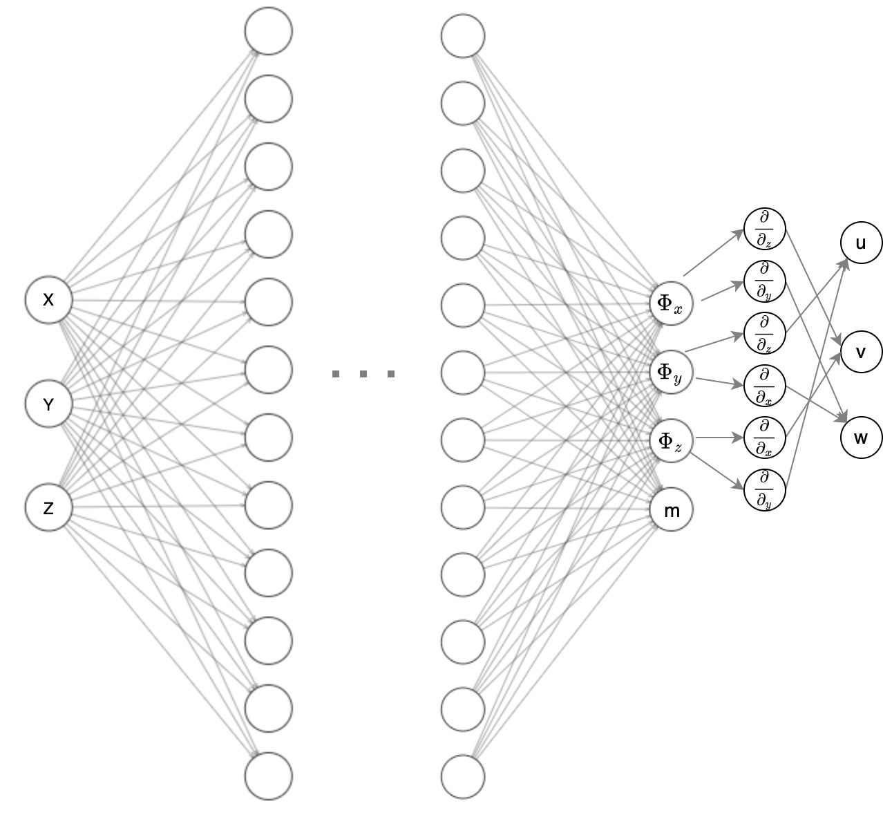
The flow velocities are modeled as a patient-specific deep neural net. The model consists of a feedforward neural network whose input are the spatial coordinates, and the output is the vector potential $$$\vec{\Phi}=(\Phi_x,\Phi_y,\Phi_z)$$$ and the MRI signal magnitude $$$m$$$. The velocity field is given by:$$\vec{V}=\nabla \times \Phi=\left(\frac{\partial \Phi_z}{\partial y}-\frac{\partial \Phi_y}{\partial z}, \frac{\partial \Phi_x}{\partial z}-\frac{\partial \Phi_z}{\partial x}, \frac{\partial \Phi_y}{\partial x}-\frac{\partial \Phi_x}{\partial y}\right)=(u, v, w)$$
The velocity definition imposes that the vector potential is itself divergence-free. Therefore, it satisfies the continuity equation automatically:
$$\nabla \cdot \vec{V}=\nabla \cdot(\nabla \times \vec{\Phi})=0$$
The loss function consists of the data fidelity term formulated by Fathi et al.11. This term considers the difference between the neural network estimated signal ( $$$S_{NN}$$$) and the original signal ($$$S_{MR}$$$ ).
$$\begin{array}{c}L=\| S_{N N}-S_{M R}||^{2}_2 \\S_{N N}=m_{N N} e^{-i 2 \pi \vec{v}_{N N}} \\S_{M R}=m_{M R} e^{-i 2 \pi \vec{v}_{M R}}\end{array}$$
We performed three experiments: simulation of a pulsatile flow (Womersley flow), computational fluid dynamics (CFD) vascular model of an aorta13, and a 4D flow acquisition of a patient with aortic coarctation. For all the experiments we used one timeframe with the highest peak flow. We used the same network architecture for each data type. The architecture had 10 hidden layers with size 25 and hyperbolic tangent activations. We trained for 500 epochs with variable learning rate (0.00025 the first 200 epochs, 0.0001 from epoch 200 to 400, and 0.00001 the last 100 epochs), batch size 100, and Adam optimizer.
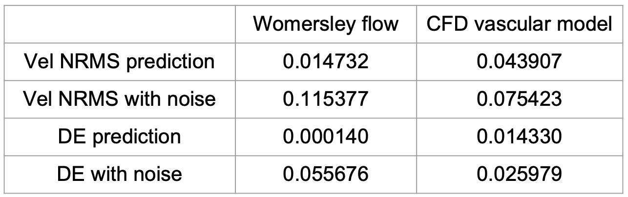
For quantitative analysis we added noise to real and imaginary parts (gaussian noise with deviation 10% of maximum real and imaginary values) of the MRI signals from Womersley flow and to the CFD vascular model. We also encoded the images using a Venc less than maximum velocity to produce aliasing artifacts ($$$0.8V_{max}$$$ for Womersley flow, $$$0.6V_{max}$$$ for CFD vascular model). To analyze the denoising performance we compute the normalize mean square velocity (VelNRMS) and the direction error (DE), defined as:
$$\begin{aligned}\operatorname{VelNRMS} &=\left(\max _i\left|v_i^r\right|\right)^{-1} \sqrt{\frac{1}{N} \sum_i\left|v_i^r-v_i^d\right|^2} \\D E &=\frac{1}{N} \sum_i\left(1-\frac{\left|v_i^r \cdot v_i^d\right|}{\left|v_i^r\right|\left|v_i^d\right|}\right)\end{aligned}$$
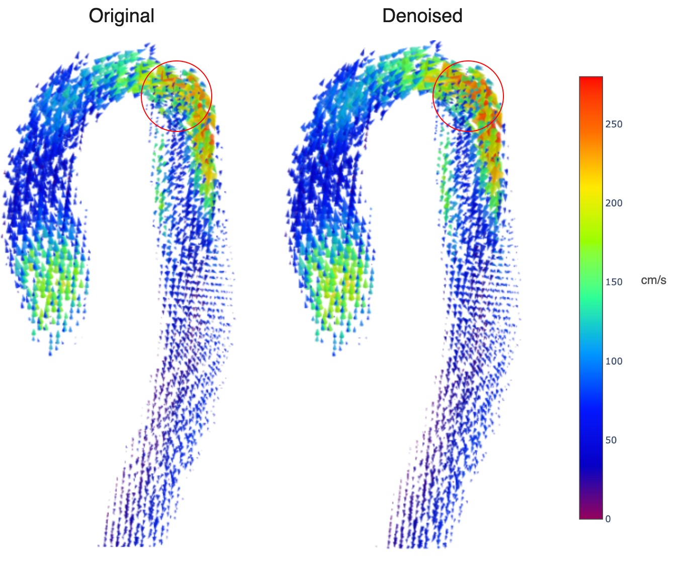
With $$$v_i^r$$$ the reference velocities and $$$v_i^d$$$ the estimated velocities. For qualitative analysis, we study the region of coarctation of the patient data as this region is more sensitive to error given the greater degree of disturbance of the aortic flow.
Results
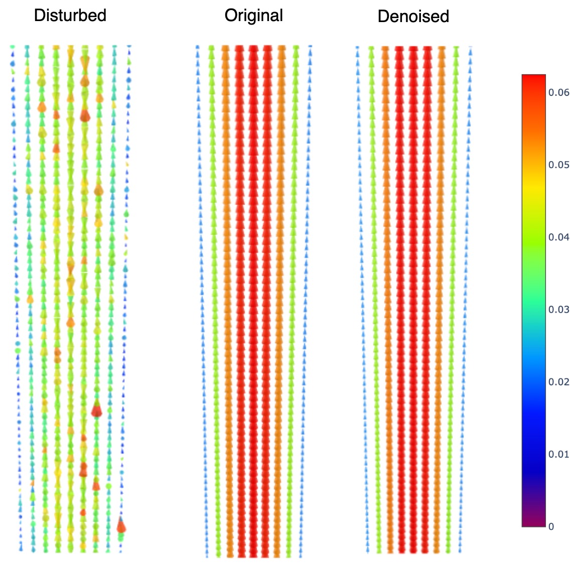
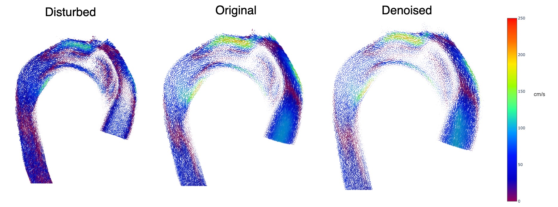
Table 1 shows the performance metrics for the predicted velocities and disturbed velocities (without aliasing). In Figures 2 and 3 we observe the aliased and disturbed velocities, the exact solutions, and the predictions. We note that the model successfully corrects the aliasing artifacts and improves the VelNRMS and DE metrics. In Figure 4 we notice that the bigger differences between the predicted and original velocity values are in the coarctation region. Similarly to Mura et al.4, near the coarctation, the divergence is locally incremented due to rapid variations in flow, which are difficult to reduce due to its amplitude and the discretization.Discussion
Our preliminary results shows that PINN with divergence-free vector potential can successfully reduce aliasing artifacts and noise in 4D flow images. Next steps of this research include a thorough comparison between similar techniques in the denoising task. Methods need to be evaluated on their ability to work on different types of data (e.g. different scanners and resolutions in healthy volunteers and patients) in a reasonable amount of processing time. In addition, we are currently working on including uncertainty quantification of model predictions (e.g with dropout as a bayesian approximation14) to ease its deployment on clinical practice.Acknowledgements
This work has been funded by ANID-PIA-ACT192064, and ANID: Millennium Science Initiative Program ICN2021_004. Also, FONDECYT # 1181057. Sotelo J. thanks to FONDECYT de iniciación en investigación 11200481. Arrieta C. was partially funded by CONICYT FONDECYT Postdoctorado 2019 #3190763. Mella H. thankfully acknowledges the financial support of the project ANID - FONDECYT Postdoctorado #3220266. PUENTE grant 2022-14 VRI, PUCReferences
1. Markl M, Frydrychowicz A, Kozerke S, Hope M, Wieben O. 4D flow MRI. Journal of Magnetic Resonance Imaging. 2012;36(5):1015-1036. doi:10.1002/jmri.23632
2. Dyverfeldt, P., Bissell, M., Barker, A. J., Bolger, A. F., Carlhäll, C. J., Ebbers, T., ... & Markl, M. (2015). 4D flow cardiovascular magnetic resonance consensus statement. Journal of Cardiovascular Magnetic Resonance, 17(1), 1-19.
3. Bostan, E., Lefkimmiatis, S., Vardoulis, O., Stergiopulos, N., & Unser, M. (2014). Improved variational denoising of flow fields with application to phase-contrast MRI data. IEEE Signal Processing Letters, 22(6), 762-766.
4. Mura, J., Pino, A. M., Sotelo, J., Valverde, I., Tejos, C., Andia, M. E., ... & Uribe, S. (2016). Enhancing the velocity data from 4D flow MR images by reducing its divergence. IEEE transactions on medical imaging, 35(10), 2353-2364.
5. Zhang, J., Rothenberger, S. M., Brindise, M. C., Scott, M. B., Berhane, H., Baraboo, J. J., ... & Vlachos, P. P. (2021). Divergence-Free Constrained Phase Unwrapping and Denoising for 4D Flow MRI Using Weighted Least-Squares. IEEE transactions on medical imaging, 40(12), 3389-3399.
6. Ong, F., Uecker, M., Tariq, U., Hsiao, A., Alley, M. T., Vasanawala, S. S., & Lustig, M. (2015). Robust 4D flow denoising using divergence‐free wavelet transform. Magnetic resonance in medicine, 73(2), 828-842.
7. Deriaz, E., & Perrier, V. (2006). Divergence-free and curl-free wavelets in two dimensions and three dimensions: application to turbulent flows. Journal of Turbulence, (7), N3.
8. Song, S. M., Napel, S., Glover, G. H., & Pelc, N. J. (1993). Noise reduction in three‐dimensional phase‐contrast MR velocity measurementsl. Journal of Magnetic Resonance Imaging, 3(4), 587-596.
9. Busch, J., Giese, D., Wissmann, L., & Kozerke, S. (2013). Reconstruction of divergence‐free velocity fields from cine 3D phase‐contrast flow measurements. Magnetic resonance in medicine, 69(1), 200-210.
10. Arzani, A., Wang, J. X., & D'Souza, R. M. (2021). Uncovering near-wall blood flow from sparse data with physics-informed neural networks. Physics of Fluids, 33(7), 071905.
11. Fathi, M. F., Perez-Raya, I., Baghaie, A., Berg, P., Janiga, G., Arzani, A., & D’Souza, R. M. (2020). Super-resolution and denoising of 4D-flow MRI using physics-informed deep neural nets. Computer Methods and Programs in Biomedicine, 197, 105729.
12. Young, D. L., Tsai, C. H., & Wu, C. S. (2015). A novel vector potential formulation of 3D Navier–Stokes equations with through-flow boundaries by a local meshless method. Journal of Computational Physics, 300, 219-240.
13. N.M. Wilson, A.K. Ortiz, and A.B. Johnson, The Vascular Model Repository: A Public Resource of Medical Imaging Data and Blood Flow Simulation Results, J. Med. Devices 7(4), 040923 (Dec 05, 2013) doi:10.1115/1.4025983.
14. Gal, Y., & Ghahramani, Z. (2016, June). Dropout as a bayesian approximation: Representing model uncertainty in deep learning. In international conference on machine learning (pp. 1050-1059). PMLR.
Figures