Synopsis

Keywords: Signal Representations, Elastography, Motion estimation, Dynamic system

We propose a framework for data-driven discovery of the governing biomechanical equations for soft tissue directly from k-space data. This framework is based on principles from Spectro-dynamics, a novel method to infer dynamical information directly from severely undersampled spectral data with high spatiotemporal resolution, and sparse regression. As a proof-of-concept, the underlying equations of motion are identified for an actively forced linear elastic system using experimentally obtained k-space data. The systems studied in this abstract are successfully identified with errors of less than 2.5% on the system parameters, and their respective displacement fields are reconstructed accurately.

Introduction

Identification of the underlying biophysical laws for soft tissue can help us to better understand their mechanical behaviour$$$^{1}$$$. Data-Driven Discovery (DDD) of the governing equations, where the underlying physics are learned from measurement data, has received a lot of attention in recent years in several engineering fields$$$^{2-5}$$$. Using the DDD approach to identify equations of motion from reconstructed MR images is not straightforward as MRI in its current form is a relatively slow modality complicating the analysis of dynamic systems at high spatiotemporal resolution. Therefore, we propose to use the recently developed Spectro-dynamic MRI framework$$$^{6}$$$ to distil the governing equations directly from k-space.
Spectro-dynamic MRI is a novel method to infer dynamical information directly from severely undersampled k-space data. This information is obtained without the use of additional devices and includes displacement fields with high spatiotemporal resolution as well as system parameters related to the mechanical properties of soft tissue. This sets the Spectro-dynamic MRI framework apart from conventional MRI scans that rely more on morphological changes for detecting disease. The envisioned applications of Spectro-dynamic MRI include the quantification of myocardial strain and stiffness which are important parameters in cardiovascular diagnostics and treatment planning.
As a proof-of-concept for data-driven discovery from k-space data, the underlying equations of motion for a dynamic phantom programmed to move like an actively forced linear elastic system are identified.

Theory

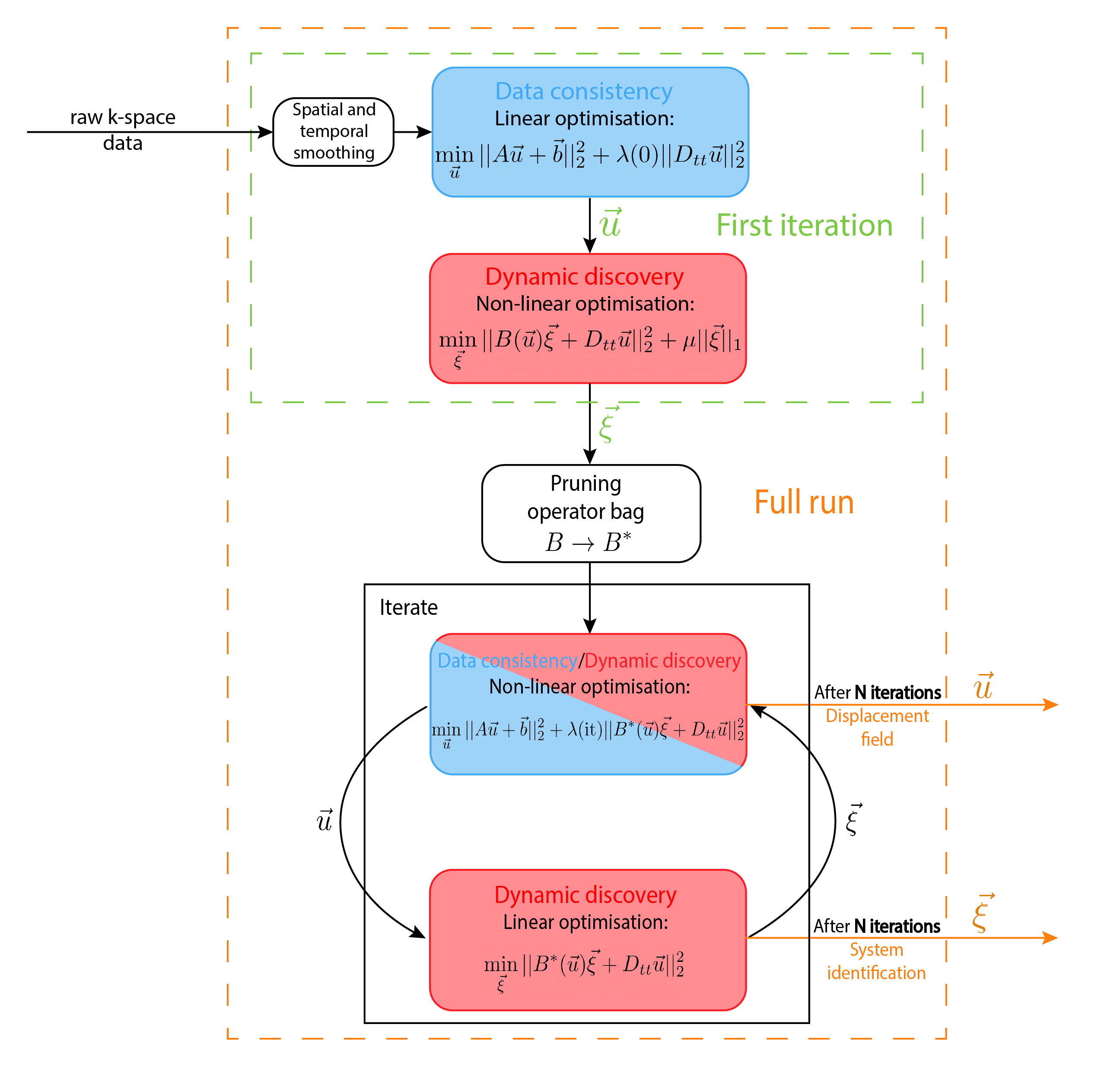
For 1D-dynamics as studied in this work, we consider the dynamic model to be of the form:$$\ddot{u}~=~f(u,\dot{u}),$$where $$$u$$$ is the displacement field. The aim of DDD is to find a closed-form analytic expression for $$$f(u,\dot{u})$$$ from the noisy measurement data. To find this analytic expression, a set of candidate basis functions are defined that $$$f$$$ might comprise of. Leveraging the data, a sparse selection of active basis functions is selected by applying sparse regression$$$^{7,8}$$$. When the displacement fields are known this results in the following minimisation problem:$$\underset{\vec{\xi}}{\arg\min}||B(\vec{u})\vec{\xi}+D_{tt}\vec{u}||_2^2+\mu||\vec{\xi}||_1,\tag{1}$$where $$$B(\vec{u})$$$ is a matrix containing the candidate basis functions as columns, $$$D_{tt}$$$ is the temporal second order finite difference operator, $$$\vec{\xi}$$$ is the sparse parameter vector that determines which basis functions are active in the model and $$$\mu$$$ the sparsity regularisation parameter. As the displacement fields are not directly available from the spectral MRI data, a model relating the k-space measurements to the displacement fields is additionally required. For this purpose, we use the measurement model from the Spectro-dynamic MRI framework, which is derived from conservation of magnetisation$$$^{6}$$$. For small deformations or rigid motion as studied in this abstract, it condenses down to the optical flow model$$$^{9}$$$. The measurement model alone is sufficient for fully sampled acquisitions but fails for highly undersampled k-space data that we consider. For this reason, a combined minimisation problem is proposed:$$\underset{\vec{u},\vec{\xi}}{\arg\min}||A\vec{u}+\vec{b}||_2^2+\lambda||B(\vec{u})\vec{\xi}+D_{tt}\vec{u}||_2^2+\mu||\vec{\xi}||_1,\tag{2}$$where the first term is the Spectro-dynamic measurement model. In this optimisation, the measurement model acts as a data consistency term while the term from eq.1 serves as a regulariser on the dynamics. The optimisation over both variables$$$(\vec{u},\vec{\xi})$$$ is performed in an iterative alternating manner. The algorithmic details are schematically depicted in Fig.1.

Methods

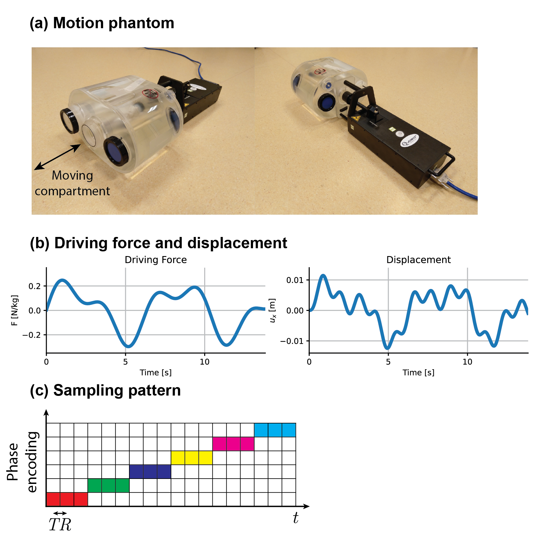
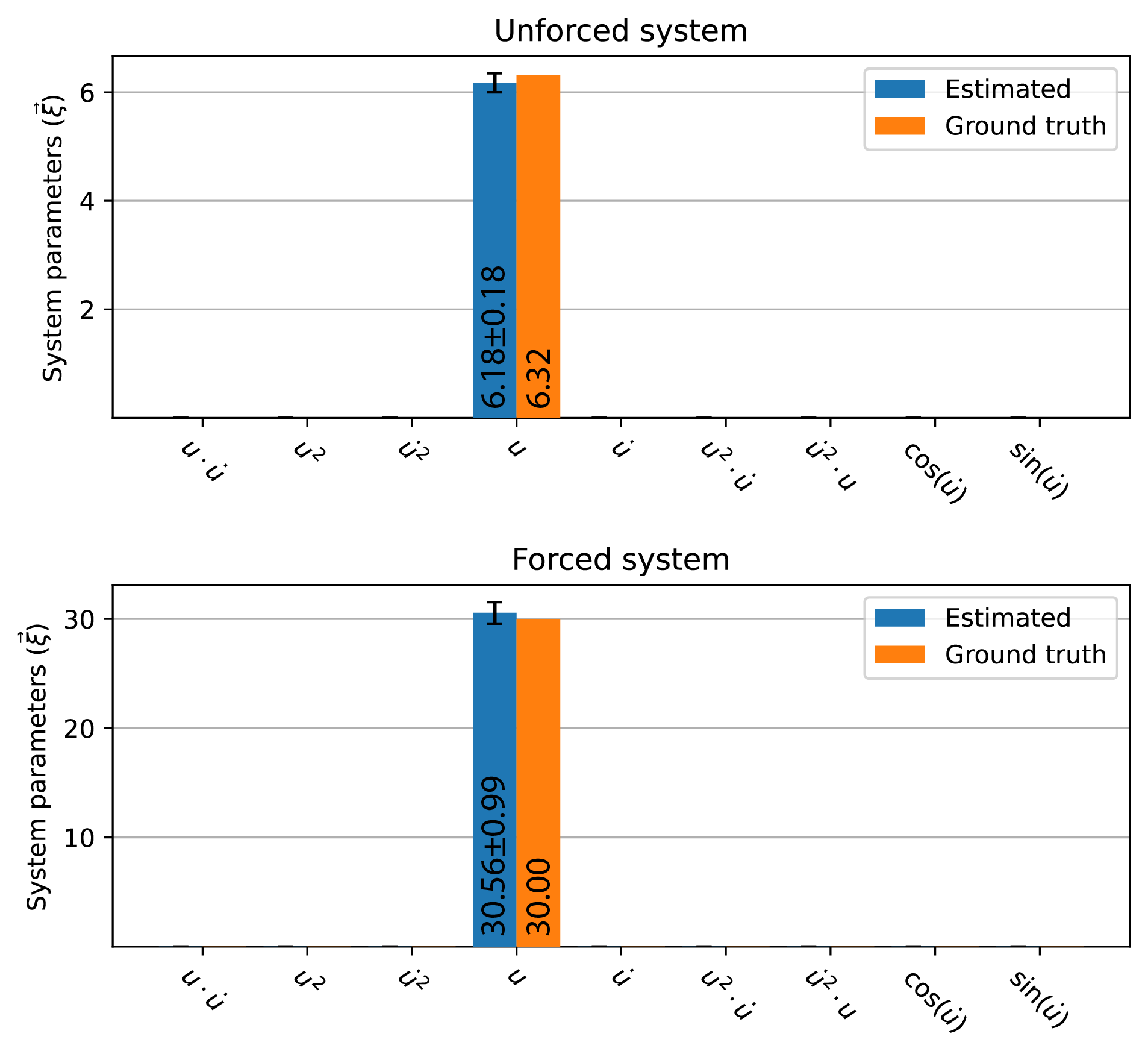
Experimental data was acquired using the Quasar MRI$$$^{4D}$$$ Motion Phantom (Modus Medical Devices Inc.) shown in Fig.2a. The moving compartment of the phantom was loaded with two gel-filled tubes (TO5, EurospinII test system). The phantom is programmed to behave as a linear elastic system with stiffness coefficient $$$k$$$ and an optional driving force $$$F(t)$$$, both normalised by the mass:$$\ddot{u}+ku=F(t)\rightarrow~f(u,\dot{u})=-ku+F(t).$$For the forced system, $$$F(t)$$$ is as shown in Fig.2b and is assumed to be known. This is a reasonable assumption for biological systems like the heart or skeletal muscles where the activation can be measured by ECG and EMG, respectively. For an unforced system, we set $$$F(t)=0$$$. The experiments were performed on a 1.5T MRI scanner (Ingenia, Philips Healthcare) with a spoiled gradient echo sequence (TE/TR=2.2/5.5ms). One slice in the coronal plane was acquired with FOV=200mmx300mm, 2mmx3mm in-plane resolution and 15mm slice thickness. To probe the motion field, 12 central phase-encode lines are repeatedly sampled 40 times in a manner characteristic for the Spectro-dynamic MRI framework(see Fig.2c) and the whole procedure is repeated 5 times for one acquisition. The reconstruction is performed using a set of 9 basis functions(see Fig.3). In order to estimate the framework's robustness, each acquisition/reconstruction is repeated 5 times.

Results

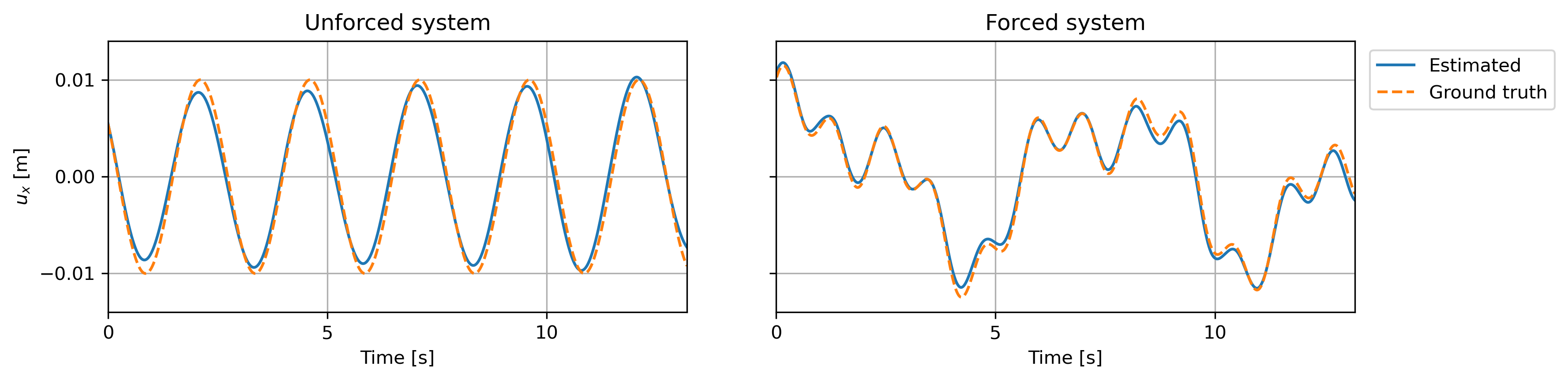
As shown in Fig.3, the correctly identified system for both experimental setups is:$$f^{*}(u,\dot{u}) = -B\vec{\xi}^{*}+F(t)=-\xi_4^{*}u+F(t).$$Notice that the estimated mass-normalised stiffness $$$\xi_4^{*}$$$ is very close to the ground truth $$$k$$$ for both systems with an error of less than 2.5%. The reconstructed displacements fields are shown in Fig.4 and are highly accurate as well.

Discussion

In this proof-of-principle study we successfully discovered mechanical models directly from k-space data. More efficient sampling patterns using grouped read-outs can further improve the accuracy and robustness of the method$$$^{10}$$$. Future research will focus on testing this framework for non-rigid motion fields in 2D and 3D. This would open up the possibility for in-vivo applications such as learning accurate phenomenological muscle models.

Conclusion

A data-driven framework to learn governing equations directly from k-space has been proposed and effectively implemented. Both the system identification as well as the reconstructed displacement fields are accurate in the presented proof-of-principle experiments.

Acknowledgements

The authors want to thank Tristan van Leeuwen for the fruitful discussions. This project is financed by the Dutch Research Council (NWO), grant 18897.