4602

A Simple Analytical Model of B₁⁺ for MRI Measurement of RF Currents in Wire-like Medical Devices

Chiara Hartmann¹, Mélina Bouldi², and Jan M Warnking¹
¹U1216, Grenoble Institut Neurosciences, Univ. Grenoble Alpes, Inserm, Grenoble, France, ²ZMT Zurich MedTech AG, Zürich, Switzerland

Synopsis

Keywords: Signal Modeling, Modelling

Safe access to MRI for patients with active implants may be possible by measuring RF currents in implants in individual patients with low-SAR sequences. We present a simple theoretical model of the B₁⁺-field close to a locally straight wire at any angle to B₀. MRI signals fitted by our model closely match magnitude and complex signals from electromagnetic simulations with a wire parallel to B₀ or tilted at 45° and magnitude experimental signals with parallel wire. RF currents reconstructed from simulated data match ground-truth values to within 6% and current profiles reconstructed from experimental signals follow simulated currents in shape.

Introduction

Patients with active implants risk thermal lesions from radio-frequency exposure during MRI due to RF currents induced in implant wires⁽¹⁾. Since RF heating depends on the individual implant configuration, patient position and landmark position, implant manufacturers specify limits of MRI exposure based on worst-case scenarios. Accurately measuring RF currents in implants in individual patients based on the B₁⁺ scattered field from the RF current in the wire using low-SAR B₁-sensitive MRI sequences may increase access to MRI for these patients.
Existing models of the B₁⁺ scattered field are limited to a wire parallel to B₀⁽²⁾, or fit background B₁ over a large region for extrapolation to the wire location, which may be difficult to achieve in patients⁽³⁾. Here we present a simple model of the B₁⁺-field close to a locally straight wire at any angle to B₀, and a validation of the model based on electromagnetic simulations and phantom experiments.

Theory

The magnitude of the linearly polarized B₁-field in an axial (x-y) plane generated by an RF current I through an infinite straight wire crossing the origin of the plane and placed at an angle ξ_j to B₀, with an azimuthal angle θ_j in the x-y plane, is:
$$\left|\overrightarrow{B}_{1,j}(r,\theta_{r})\right|=\frac{\mu_{0}\mu_{r}I\cos\xi_{j}}{2\pi r\left(1-\sin²\xi_{j}\cos²\left(\theta_{r}-\theta_{j}\right)\right)},$$
with (r,θ_r) cylindrical coordinates in the x-y plane, μ₀the permeability of free space and μ_rthe relative permeability of the medium surrounding the wire.
The total transmit field B₁⁺ is the left circularly polarized component of the phased sum of the background B₁⁺ field generated by the MRI (B_1,b⁺) and B_1,j:
$$ \left|B_{1}^{+}\left(r,\theta_{r}\right)\right|=B_{1,b}^{+}\left\{ 1+\left(\frac{\left|\overrightarrow{B}_{1,j}(r,\theta_{r})\right|}{2B_{1,b}^{+}}\right)^{2}+\frac{\left|\overrightarrow{B}_{1,j}(r,\theta_{r})\right|}{B_{1,b}^{+}}\sin\left(\phi'_{j}-\theta_{r}\right)\right\} ^{1/2}$$
$${\measuredangle}B_{1}^{+}\left(r,\theta_{r}\right)=-\phi_{b}+\measuredangle\left(\frac{\frac{\left|\overrightarrow{B}_{1,j}(r,\theta_{r})\right|}{B_{1,b}^{+}}\cos\left(\phi'_{j}-\theta_{r}\right)}{2+\frac{\left|\overrightarrow{B}_{1,j}(r,\theta_{r})\right|}{B_{1,b}^{+}}\sin\left(\phi'_{j}-\theta_{r}\right)}\right),$$
with φ_b the phase of B_1,b, φ_j the phase of I and φ'_j=φ_j-φ_b. |B_1,b⁺| and φ_b are considered constant in space close to the wire.

Methods

The Model was validated in simulations and phantom experiments, using an ASTM Phantom⁽⁴⁾ containing HEC gel, and a straight 20-cm copper wire of 3mm diameter, insulated along the length and bare at both tips.
Harmonic EM simulations were performed using Sim4Life (ZMT, Zürich, Switzerland) with a model of the RF transmit coil in our MRI tuned to 128MHz⁽⁵⁾. The wire was placed either parallel to B₀ or tilted at 45° in a horizontal plane, at 26mm from the lateral wall and 46mm from the bottom of the phantom. We extracted the complex wire current and the complex B₁⁺-field close to the wire inside the phantom (Fig.1) in 41 axial planes at 5-mm intervals along the wire. From B₁⁺, MRI signals were simulated in each plane using analytical signal equations for two AFI sequences (see parameters below). B_1,b was estimated from a simulation without wire.
MRI experiments were performed in an Achieva dStream 3.0T TX (Philips, Netherlands) at IRMaGe MRI facility (Grenoble, France). Data from two AFI sequences were combined (4 images in total) to increase the B₁ dynamic range⁽⁶⁾. 16 axial slices were acquired at 11,4-mm intervals along a wire parallel to B₀. AFI sequence parameters were α=46.7°, TR₁=15.6 ms, n=1.09 and α=32.2°, TR₁=25.3 ms, n=9.6, with 2x2-mm in-plane voxel size.
The analytical model of the B₁⁺-field coupled to AFI signal equations was used to fit the model parameters using differential evolution⁽⁷⁾, minimizing the RMS difference between modeled MRI signals and simulated or acquired ones over a patch of 12x12 voxels around the wire (576 signals from 4 AFI images). Simulated data were fitted based on magnitude or complex MRI signals; acquired data were fitted based on magnitude only. To compare simulations and phantom experiments, I was normalized to a local reference B_1,ref=3.1µT: $$$I_{ref}=I\cdot{B_{1,ref}}/{B_{1,b}}$$$.

Results

Model parameters obtained by fitting MRI signals from EM simulations closely matched the ground-truth values extracted from simulations for both the wire parallel to B₀ (Fig.2) and the tilted wire (Fig.3). Average relative error of the current estimation along the wire was 3.6% from complex and 2.5% from magnitude signals for the wire parallel to B₀ and 5.6% (complex) and 4.8% (magnitude) for the tilted wire. Fitting complex MRI signals did not improve the accuracy of parameters estimates, except for φ'_j (Figs.2c/3c). Modeled MRI signals closely matched those from simulations, with a median relative difference of 1.2% for complex and 3.4% for magnitude signals for the wire parallel to B₀, and 2.2% (complex) and 6.3% (magnitude) for the tilted wire.
The current amplitude along the wire obtained by fitting experimental data followed a shape closely matching the profile obtained in simulations (Fig.4). The median relative difference between acquired and modeled magnitude MRI signals was 5.2%.

Discussion & Conclusion

The results showed very good agreement between EM simulations and our analytical model, even close to the tips of the wire, where a discrepancy is expected due to the hypothesis of an infinitely long wire in the model. Experimental data was fitted well, with a current profile closely matching simulations. We observed however a significant difference in current amplitude between simulations and experiments, despite current fits from acquisition and simulations being scaled to the same reference B_1,b-value of 3.1µT. Since we could not measure RF currents in the experiment, the origin of this difference remains unclear. Future work will aim to validate the RF currents in the experiments and to optimize the acquisition for lower SAR and shorter duration.

Acknowledgements

This work was performed on the IRMaGe platform member of France Life Imaging network (grant ANR-11-INBS-0006). Chiara Hartman receives a PhD grant from Université Grenoble Alpes.

References

⁽¹⁾ Jörg Spiegel, Gerhard Fuss, Martin Backens, Wolfgang Reith, Tim Magnus, Georg Becker, Jean-Richard Moringlane, and Ulrich Dillmann. “Transient Dystonia Following Magnetic Resonance Imaging in a Patient with Deep Brain Stimulation Electrodes for the Treatment of Parkinson Disease: Case Report.” Journal of Neurosurgery 99, no. 4 (October 2003): 772–74. https://doi.org/10.3171/jns.2003.99.4.0772.

⁽²⁾Michiel R. van den Bosch, Marinus A. Moerland, Jan J. W. Lagendijk, Lambertus W. Bartels, and Cornelis A. T. van den Berg. “New Method to Monitor RF Safety in MRI-Guided Interventions Based on RF Induced Image Artefacts: Method to Monitor RF Safety in MRI-Guided Interventions.” Medical Physics 37, no. 2 (January 26, 2010): 814–21. https://doi.org/10.1118/1.3298006.

⁽³⁾ Janot P. Tokaya, Alexander J.E. Raaijmakers, Peter R. Luijten, Alessandro Sbrizzi, and Cornelis A.T. Berg. “MRI-Based Transfer Function Determination through the Transfer Matrix by Jointly Fitting the Incident and Scattered Field.” Magnetic Resonance in Medicine 83, no. 3 (March 2020): 1081–95. https://doi.org/10.1002/mrm.27974.

⁽⁴⁾ F04 Committee. “ASTM F2182-19e Test Method for Measurement of Radio Frequency Induced Heating On or Near Passive Implants During Magnetic Resonance Imaging.” ASTM International, 2019. https://doi.org/10.1520/F2182-19E01.

⁽⁵⁾ Mélina Bouldi, and Jan M Warnking. “EM and Thermal Validation of a Numerical Elliptical Birdcage at 3T in the Presence of a Long Conductive Wire.” In Proceedings of the Joint Annual Meeting ISMRM-ESMRMB 2014, 6672. Milan, Italy, 2014.

⁽⁶⁾ Mélina Bouldi, Tatiana Nemtanu, and Jan M Warnking. “High-Dynamic-Range High-SNR B1+ Mapping Using Multiple Cyclic MR Signals.” In Proceedings of the ISMRM 25th Annual Meeting, 347. Honolulu, HI, 2017.

⁽⁷⁾ Swagatam Das, and Ponnuthurai Nagaratnam Suganthan. “Differential Evolution: A Survey of the State-of-the-Art.” IEEE Transactions on Evolutionary Computation 15, no. 1 (2011): 4–31. https://doi.org/10.1109/TEVC.2010.2059031.

Figures

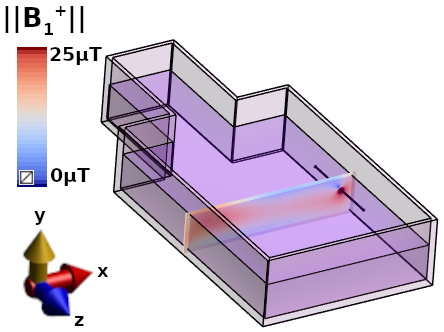
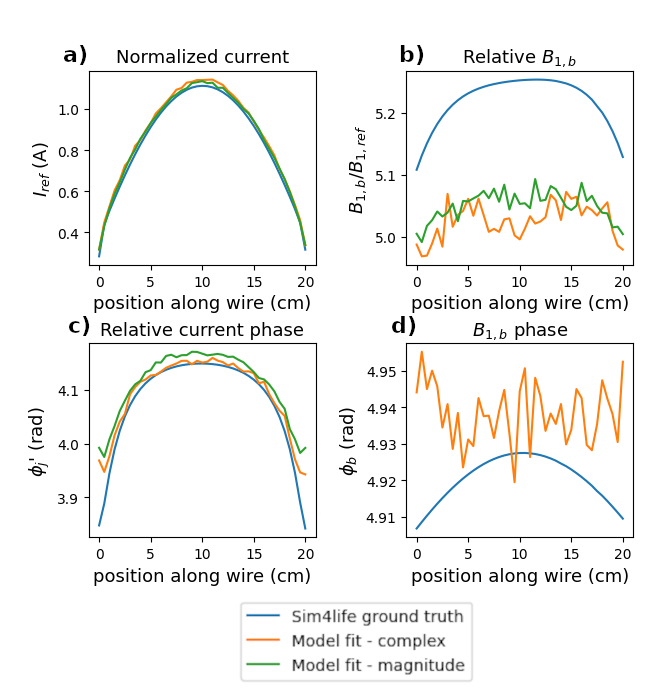
Fig.1: Configuration used for validation of the model of the B₁⁺-field around a wire. The same configuration was used for 3D EM simulations of B₁+ performed using Sim4Life (ZMT, Zürich, Switzerland) and MRI acquisitions. A wire tilted at 45° in the x-z plane was also tested in simulations.

Fig.2: Configuration with the wire parallel to B₀

Simulated (ground truth) values of several model parameters (blue curves), and corresponding values derived by fitting our analytical model to the simulated MRI signals (orange curves for fitting complex MRI signals, green curves for fitting magnitude MRI signals).

a) RF normalized current in the implant wire;

b) Value of background B₁ (B_1,b) relative to a reference B₁ of 3.1µT;

c) Phase of the wire current relative to the background B₁ phase;

d) Background B₁ phase (fitted only for complex signals)

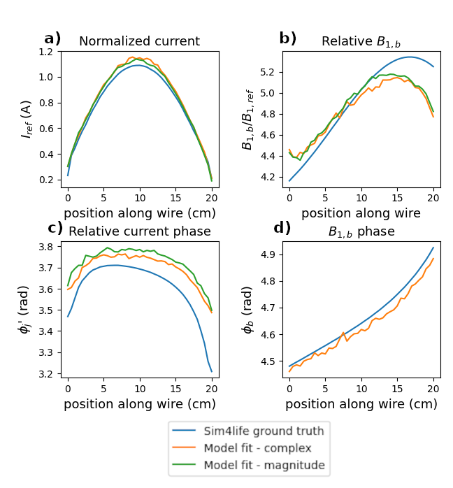
Fig.3: Configuration with the wire at a 45° angle with respect to B₀

a) RF normalized current in the implant wire;

b) Value of background B₁ (B_1,b) relative to a reference B₁ of 3.1µT;

c) Phase of the wire current relative to the background B₁ phase;

d) Background B₁ phase (fitted only for complex signals)

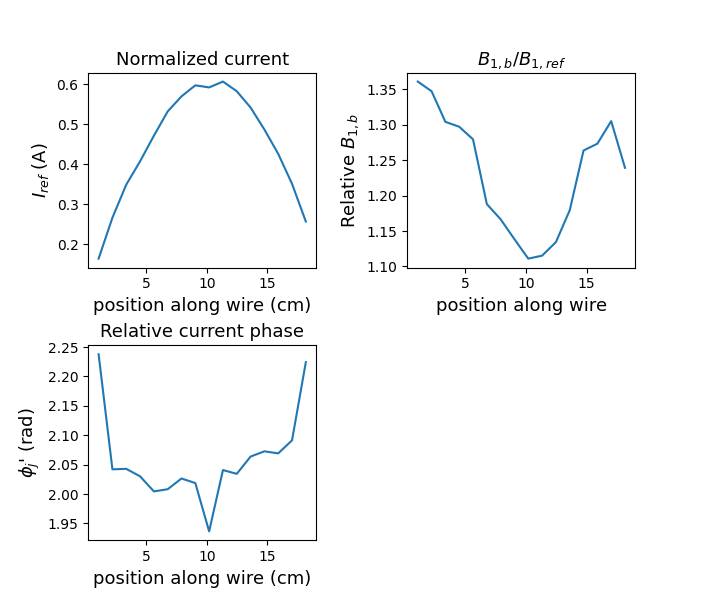
Fig.4: Configuration with the wire parallel to B₀

Model parameter values derived by fitting our analytical model to acquired magnitude MRI signals

a) RF normalized current in the implant wire;

b) Value of background B₁ (B_1,b) relative to a reference B₁ of 3.1µT;

c) Phase of the wire current relative to the background B₁ phase

Proc. Intl. Soc. Mag. Reson. Med. 31 (2023)

4602

DOI: https://doi.org/10.58530/2023/4602