Synopsis

Keywords: Gradients, New Devices, Insert gradient coil

A compact, lightweight device that generates a strong nonlinear gradient was recently developed for prostate DWI. In principle this hardware can be installed/removed for individual scans, but an additional question is whether the gradient field would need to be mapped and characterized with each installation. This work shows high reproducibility of the field after different installations, implying a single high quality field map can be reused. This result paves the way for practical clinical use of this insert gradient.

Introduction

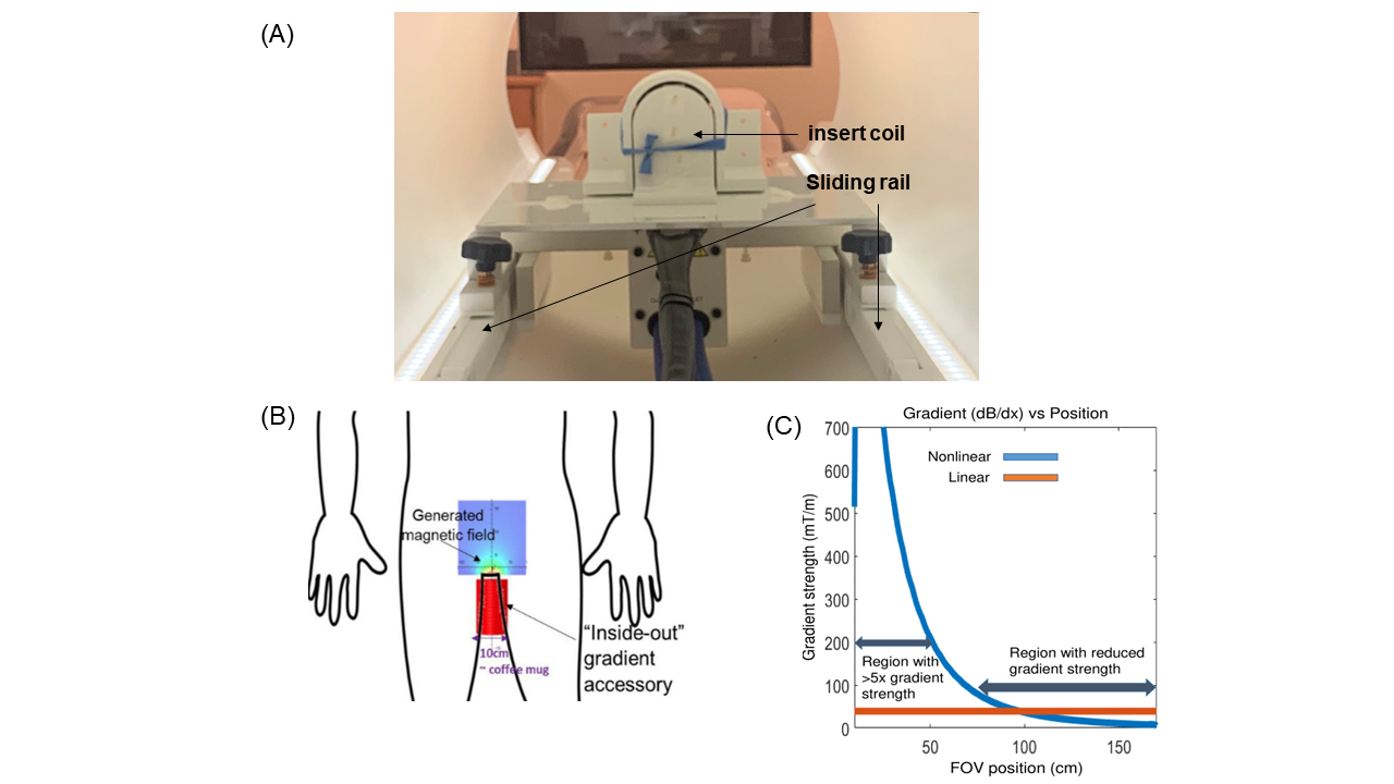
The gradient amplitude used in Diffusion Weighted Imaging (DWI) plays a crucial role in the Signal-to-Noise Ratio (SNR), diffusion contrast, and other factors of image quality. Many design schemes have been reported to increase the gradient strength¹, including insert coils which can allow for increased efficiency, gradient strength, and slew rate. However, most previous insert gradients for human imaging have been relatively heavy, typically installed on a semi-permanent basis².

We recently proposed a compact (10 cm diameter) “inside-out” nonlinear gradient coil for prostate DWI which can be installed and removed on a scan-by-scan basis³. By focusing the gradient over a prostate ROI, the nonlinear gradient coil allows for higher inductance and reduces the voltage required for the slew rate. It achieves ~500mT/m over the intended ROI, and the limited spatial extent of the field is also expected to mitigate peripheral nerve stimulation.

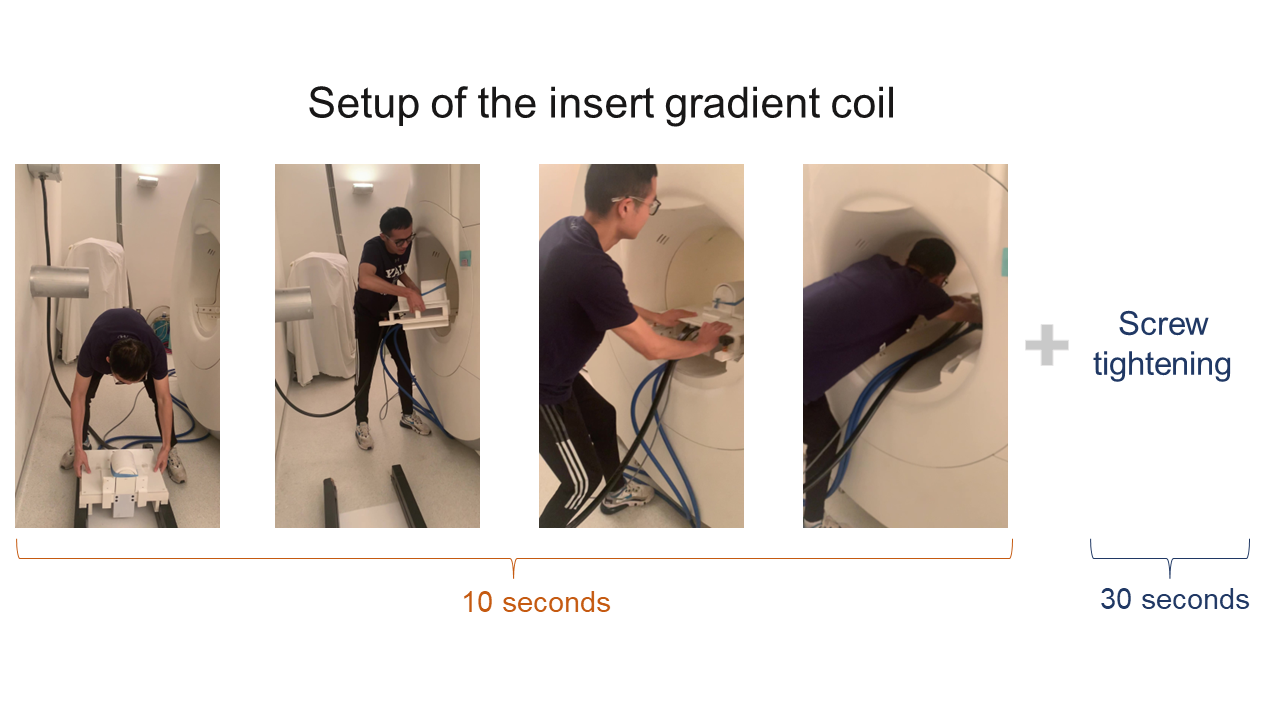
Because the coil is smaller and lighter than many insert gradients for clinical use, the installation can be completed by one person in under a minute. However, given this rapid installation, there is concern that the generated field may vary with each installation, which would require field mapping prior to each scan. Here we demonstrate the reproducibility of the field map which suggests field maps can be reused with no appreciable loss in accuracy. This implies the device can be ready for immediate DWI scanning following the quick installation.

Method

The presented insert gradient coil was designed and manufactured by Tesla Engineering Ltd (Storrington, England, UK). A sliding rail was installed inside the scanner’s bore and two holes were drilled to fix the gradient coil. Fig. 2 illustrates the setup with a series of pictures. It takes around 40 seconds to lift the gradient coil, push it to the isocenter of the scanner, and fix the position by tightening the screws. This relatively simple securing process greatly increases the reproducibility of hardware positioning.

Three water bottles were arranged to measure the field over a range of locations. All processing was masked to the occupied space in the volume. 3D Gradient Echo (GRE) with a bipolar nonlinear gradient waveform of the insert coil was used for field mapping, with unbalanced bipolar trapezoidal gradients at equal magnitude. Three volumes were acquired, incrementing the duration of the second gradient pulse to achieve different levels of field-dependent winding. The phase difference between the volumes was used for field map calculations. Imaging parameters were as follows: FOV=450x450x128mm³; resolution=1.56x1.56x1.60mm³; TR=20.0ms; TE=6.5ms. A coronal slice through the insert gradient coil and a transversal slice in front of it were analyzed to assess the reproducibility. The field mapping experiments were repeated 4 times. The coil was removed and then pushed back between each mapping experiment.

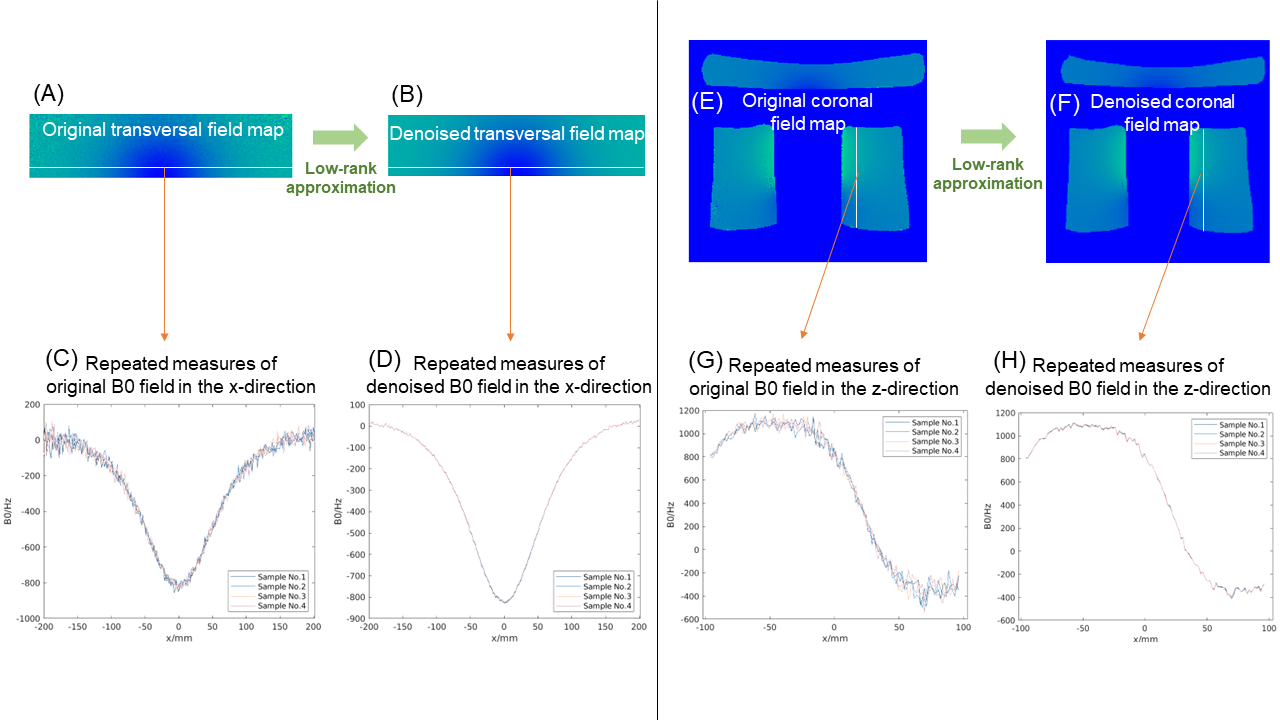
The true field map is expected to be smooth and thus low-rank. This was exploited to denoise each field map measurement and capture the underlying B0 profile. Specifically, we used a low-rank approximation based on Singular Value Decomposition (SVD), as it yields the most accurate low-rank approximation in a least-squares sense, given a certain rank⁴. Adjacent slices formed a group of samples for SVD and the first 2 singular vectors were selected to generate denoised field maps, i.e. rank-2 SVD truncation. Notably, the denoising was performed separately and independently for the field map volume from each experiment.

Results and Discussion

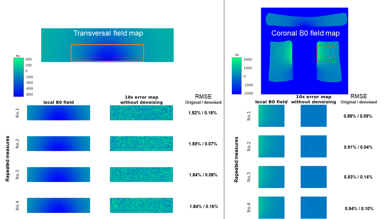
Fig. 3 shows typical transversal (A) and coronal (E) field maps. Coronal field maps are shown masked to the occupied region, while transverse slices are cropped to the occupied region. Based on rank-2 SVD truncation, the denoised maps (B, F) have smoother profiles and are believed to better reflect the true field map. To investigate the B0 profile, one line across the effective space was selected for each view with and without denoising. The repeated 4 measures of the field in the x-direction (C, D) and the z-direction (G, H) were plotted. The 4 samples demonstrate similar profiles of the field, especially in the denoised field maps.

Fig. 4 is a quantitative demonstration of two selected ROIs in the transversal and coronal views, respectively. Using the denoised error maps, the average of 4 measures was taken to be the standard field map and we show the 10x error maps for each experiment as deviations from this mean field. The 10x error map does not exhibit significant field profiles other than noise, implying that field shape and amplitude were consistent across runs within the field map measurement error. We also report the normalized Root Mean Square Error (RMSE). For both transversal and coronal local fields, the normalized RMSEs are below 2% for original field maps and below 0.2% for denoised field maps. This implies that deviations in the b-value resulting from previously acquired maps will be very low, with essentially no impact on DWI imaging.

Conclusion

The reproducibility of the field map is demonstrated for an easily installed/removed nonlinear gradient coil for prostate MRI, implying that premeasured maps can be reused. It is therefore feasible to install/remove this gradient for individual scan sessions, with no need for a customized field map acquisition.

Acknowledgements

No acknowledgement found.