Synopsis

Keywords: Phantoms, Velocity & Flow, Simulation

The lattice Boltzmann method (LBM) is a versatile technique to simulate fluid dynamics in complex environments. We extended the LBM to flows with a spin 1/2 degree of freedom in external magnetic fields. We performed 3D simulations for FLASH MRI of a laminar flow in a pipe and the complex flow of the Karman vortex street.

Introduction and Purpose

Flow related imaging artifacts in MRI are not fully understood in scenarios with complex flow. Extending previous numerical techniques [1], the proposed lattice Boltzmann method (LBM) [2] is able to simulate combined flow, diffusion, and magnetization of flowing proton.

Previously, we showed results from a 3D LBM with a joint velocity-spin distribution and verified basic properties for laminar flow [3]. The simulation required the use of small timesteps to accurately capture the dynamics of the Bloch equation. To be able to apply this method in more complex scenarios, we exploit precomputed state-transition matrices [4] for solving the Bloch equations between larger time steps sufficient for simulation of fluid dynamics.

Therefore, we can now validate the predicted in-flow effect in a 3D laminar pipe flow for a FLASH sequence with experimental results reported previously [5]. We also qualitatively compare numerical and experimental results for FLASH MRI of a Karman vortex street.

Theory

We previously proposed an extension of the classical LBM by changing the velocity distribution $$$f(\vec{r}, \vec{c}, t)$$$ into a matrix-valued semi-classical velocity-spin distribution $$$D(\vec r, t)$$$ of flowing spin 1/2 particles [5]. With the particle velocity $$$\vec{c}$$$, spatial location $$$\vec{r}$$$ and time step $$$t$$$. The velocity-spin distribution $$$D(\vec r, \vec{c}, t)$$$ can be discretized by:
$$D_i(\vec r, t) := \frac{1}{2} \sum_j f_{i,j}(\vec r, t) \sigma_j, $$
where we make use of the expansion of a quantum mechanical density operator $$$D$$$ of 1/2 particles into the Pauli matrices $$$\sigma_j$$$ and identitiy matrix $$$\sigma_0$$$. The indices $$$j$$$ and $$$i$$$ denote the polarization direction {$$$0,x,y,z$$$} and discrete direction {$$$0,x,y,z$$$} of the particle velocity $$$\vec{c}_i$$$. The macroscopic quantities can be computed from the expectation values of the distribution. This leads to the magnetization $$$\vec{M}$$$, density $$$\rho$$$ and velocity $$$\vec{u}$$$:
$$\rho = \sum_i f_{i,0}, \qquad \rho \vec u = \sum_i f_{i,0} \vec c_i, \quad \text{ and } \quad M_j = \sum_i f_{i,j} \text{ .}$$
The LBM simulates the discrete Boltzmann equation by separated streaming and collision steps [5]. During streaming each $$$f_{i,j}$$$ is streamed forward to the next lattice node along its direction $$$\vec c_i$$$. In the collision step, $$$f_{i,j}$$$ is redistributed onto a local equilibrium distribution $$$f^{eq}_{i,j}(\rho, \vec{u})$$$. To model a step of the time-discretized Bloch equations an additional Bloch step is applied during collision.

To be able to increase the step size, we replaced traditional Bloch simulation with hard pulses by precomputed state-transition matrices for larger steps. The state-transition matrices model relaxation and the effects of the external magnetic fields and can be reused for the RF excitation in each TR.

Methods

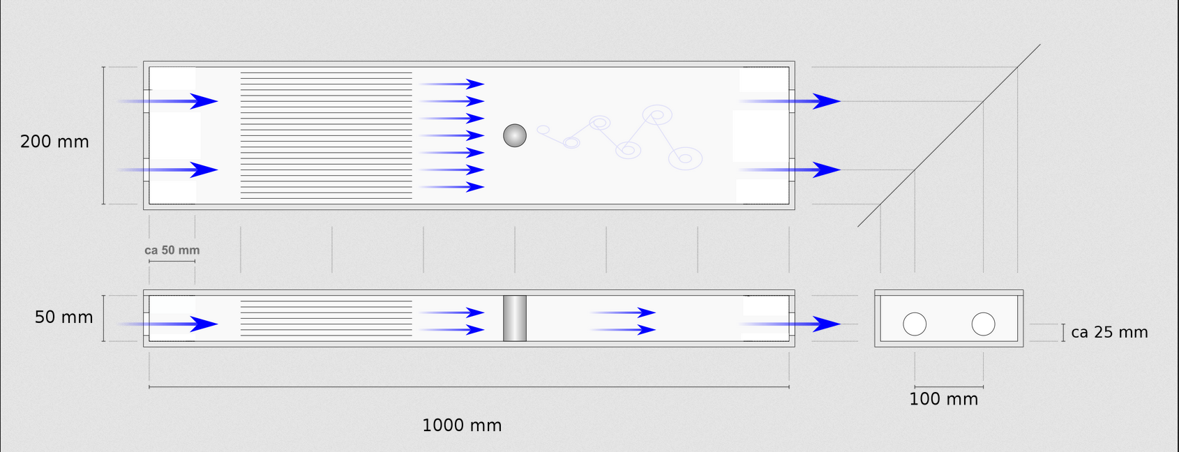
To validate the signal change due to in-flow effects in a developing laminar pipe flow, the excitation by a spoiled phase contrast FLASH sequence (TR = 11ms, TE = 9.47ms, VENC = 4) at the middle of a pipe was simulated on a [31/31/151] grid and also measured experimentally in a flow phantom. At the in- and outflow Zhu-He velocity and interpolation boundaries were utilized [2] and at the wall a staircase approximation with diffuse reflection boundaries was used [3]. Simulations were performed for varying velocity, slice thickness and flip angle. The signal intensities are validated using previous experimental results reported in [3].

Data for the Karman vortex street was acquired using a laminar flow phantom [6] as sketched in Figure 1 with a radial FLASH sequence (TR = 2.3ms, TE = 1.29ms, FA = 8°, resolution: 2mm, slice thickness 7mm, matrix size 128x128, 41 spokes per frame with 5-turn scheme, two-fold oversampling) and calculated with a nonlinear inverse reconstruction [7]. The simulation was conducted on a [51/31/196] grid with the same Reynold number as the flow phantom.

All simulations were run in parallel on a AMD Ryzen 7 5800-x processor with 8 kernel.

Results

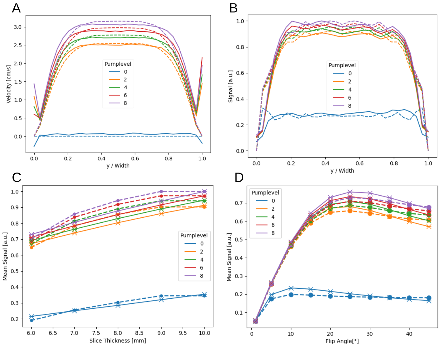
With the precomputed state-transition matrices a speedup from 10h to 2:30h was obtained for the [31/31/151] grid.

Figure 2 shows the numerical (dotted) and experimental (solid) results for the pipe flow. The cross-sectional velocity and signal profiles at the central plane of the pipe for different pump-levels are shown in (A) and (B). (C) and (D) show the change of the 3D cross-sectional mean signal for varying slice thickness and flip angle. The (mean) signals are scaled by the maximum (mean) signal appearing in the measurement and the simulation.

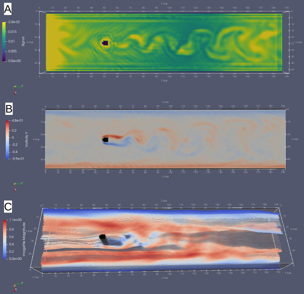
Figure 3 depicts the signal (A), vorticity in Y (B) and streamlines (C) of the simulated Karman vortex street.

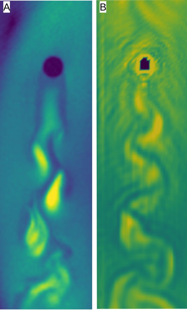
Figure 4 shows the simulated signal at a selected time point (A) and an experimental image (B).

Discussion and Outlook

We validated a method for simulating combined spin and fluid physics in 3D. We further accelerate the simulation by a factor of four using precomputed state-transition matrices. For the signal predicted for the in-flow effect in FLASH MRI for laminar pipe flow, the numerical results correspond well to experimental results. Moreover, we show the simulations of the complex signal behavior in the Karman vortex street, which qualitatively agree with experimental results.

References

[1] Jurczuk K., Kretowski M., Bellanger J., Eliat P., Saint-Jalmes H., Bézy-Wendling J. (2013) Computational modeling of MR flow imaging by the lattice Boltzmann method and Bloch equation. In Mag. Res. Imag. Vol 31; 7; 2013.
[2] Krüger T., Halim K. (2017) The Lattice Boltzmann Method, Springer-Verlag.
[3] Adler A., Schaten P., Wang Y., Uecker M. (2022) 3D-Simulation of Flowing Spins using the Lattice Boltzmann Method with Maxwell Diffuse Reflection Boundaries. ISMRM 2022. In Proc. Intl. Soc. Mag. Reson. Med. 30; 1227.
[4] Scholand N., Graf C., Uecker M. (2022) Efficient Bloch Simulation Based on Precomputed State-Transition Matrices. ISMRM 2022. In Proc. Intl. Soc. Mag. Reson. Med. 30; 0748.
[5] Adler A., Kollmeier J., Scholand N., Rosenzweig S., Wang Y., Uecker M. (2021) Simulation of Flowing Spins in MRI using the Lattice Boltzmann Method. ISMRM 2021. Proc. Intl. Soc. Mag. Reson. Med. 29; 2100.
[6] Kollmeier, J.M. "Multi-Directional Phase-Contrast Flow MRI in Real Time." PhD diss., Georg-August-Universität Göttingen, 2020.
[7] Uecker M., Hohage T., Block K.T., Frahm J. (2008) Image reconstruction by regularized nonlinear inversion--Joint estimation of coil sensitivities and image content. Magn Reson Med. 60:674-82.