4570

Characterizing gradient performance and estimating Maxwell fields at 0.55T.

Daniel West¹, David Leitão¹, Raphael Tomi-Tricot^1,2, Tobias C Wood³, Jo Hajnal^1,4, and Shaihan Malik^1,4
¹Biomedical Engineering, King's College London, London, United Kingdom, ²MR Research Collaborations, Siemens, Frimley, United Kingdom, ³Department of Neuroimaging, King's College London, London, United Kingdom, ⁴Centre for the Developing Brain, King's College London, London, United Kingdom

Synopsis

Keywords: System Imperfections: Measurement & Correction, Gradients

In this work we use a general sequence to characterize gradient imperfections at low field (0.55T) by measuring the gradient impulse response function (GIRF). Maxwell fields become non-negligible at lower field strengths and so we incorporate these into our GIRF calculation to form a single processing pipeline. Once the predictive ability of the GIRF was confirmed, we use our data to estimate the Maxwell phase and compare this to an analytic approach; good agreement is observed. These results will inform future low-field investigations and enable an improved image quality for sequences that are particularly prone to gradient imperfections.

Introduction

The gradient performance of commercial MR systems is imperfect due to factors such as: time delays, eddy currents and mechanically induced field oscillations. To characterize these distortions, NMR field probes^1,2 can be used and although accurate, these devices are expensive and not readily available. Gradient impulse response functions (GIRFs) assume that the gradient chain is a linear time-invariant system and have often been shown to be a sufficient surrogate for field probes^3,4. GIRF calculation is performed by measuring the response of the gradient system using a combination of input waveforms. The response of the gradient system itself could be measured using field probes⁴ or imaging-based methods such as the thin-slice method^3,5–7. This technique is usually limited to providing zeroth-order and first-order self-terms but cross-terms can also be determined⁸.

Beyond the imperfections mentioned above, MRI gradients are accompanied by higher-order spatially varying fields known as concomitant (Maxwell) fields. These are often neglected during MR experiments but become more significant at lower field strengths due to an inverse linear dependence on magnetic field strength. Quantification of their impact becomes important in low-field MRI and correction strategies have previously been proposed⁹though here, Maxwell terms were derived from gradient terms and not measured directly. In this work we use a spatially resolved gradient measurement method¹⁰ to characterize GIRFs and extend this to measure Maxwell terms from a single acquisition. We demonstrate its effectiveness on data acquired at 0.55T.

Theory

The phase evolution during the sequence in Figure 1 can be described by Equation 1:

$$[1]\;\phi(x,y,t)=\mathrm{\mathbf{x}}\cdot\mathrm{\mathbf{k}}+\gamma B_0t+\phi_{\mathrm{C}}$$

$$$\phi$$$ is a matrix with dimensions of number of pixels ($$$\mathrm{N_p}$$$) by the number of timepoints ($$$\mathrm{N_t}$$$), $$$\mathrm{\mathbf{x}}$$$ is a position matrix that has dimensions $$$\mathrm{N_p}\times3$$$ and $$$\mathrm{\mathbf{k}}$$$ is a $$$3\times\mathrm{N_t}$$$ matrix that is related to the actual gradient waveform by Equation 2:

$$[2]\;\mathrm{\mathbf{k}}=\gamma\mathrm{\mathbf{g}}\left[\begin{matrix}1&1&1&...&1\\0&1&1&...&1\\0&0&1&...&1\\...&...&...&...&...\\0&0&0&...&1\end{matrix}\right]\Delta t=\gamma\mathrm{\mathbf{g}}\mathrm{\mathbf{A}}\Delta t$$

where $$$\mathrm{\mathbf{g}}$$$ has dimensions $$$3\times\mathrm{N_t}$$$ and $$$\mathrm{\mathbf{A}\Delta}t$$$ is an integration matrix with dwell time $$$\Delta t$$$. $$$\phi_{\mathrm{C}}$$$ is the phase evolution due to concomitant fields and is given by Equation 3:

$$[3]\;\phi_{\mathrm{C}}=-\gamma\mathrm{\mathbf{B_C}}\mathrm{\mathbf{A}}\Delta t$$

where:

$$[4\mathrm{a}]\;\mathrm{\mathbf{B_C}}=\sqrt{B_x^2+B_y^2+B_z^2}-B_z$$
$$[4\mathrm{b}]\;B_x=-0.5g_zx+g_xz$$
$$[4\mathrm{c}]\;B_y=-0.5g_zy+g_yz$$
$$[4\mathrm{d}]\;B_z=B_0+g_xx+g_yy+g_zz=B_0+\mathrm{\mathbf{g}}\cdot\mathrm{\mathbf{x}}$$

Methods

Experiments were completed on a clinical 0.55T scanner (MAGNETOM Free.Max, Siemens Healthcare, Erlangen, Germany) and a large disc-shaped MR system water phantom was used for all measurements (4.6x4.6x10mm resolution, single-slice, TR = 20ms, TE = 5ms, FOV = 440mm). This phantom was scanned in all three orientations with two phase-encoding axes (Figure 1) such that all cross-terms could be estimated. As per previous work⁸, a variable amplitude chirp waveform was used as our test waveform with a duration of 10ms and maximum amplitude of 2mT. Its amplitude was varied so that we could operate at the maximum slew rate limit of the scanner.

Image phase was normalized by the phase of an image acquired without a chirp waveform and then used to compute $$$\mathrm{\mathbf{g}}$$$ using the steps outlined above. Typical GIRFs were calculated using Equation 5:

$$[5]\;H=\frac{\mathcal{F}(\mathrm{\mathbf{g}})}{\mathcal{F}(\mathrm{\mathbf{g_{nom}}})}$$

where $$$\mathcal{F}$$$ denotes the Fourier transform in the time dimension and $$$\mathrm{\mathbf{g_{nom}}}$$$ is the nominal input gradient waveform. We estimate the corresponding Maxwell phase from Equation 6 where $$$h=\mathcal{F}^{-1}H$$$:

$$[6]\;\hat\phi_{\mathrm{C}}=\phi_{\mathrm{meas}}-(\mathrm{\mathbf{g_{nom}}}\ast h(t))-\gamma B_0 t$$

$$$\phi_{\mathrm{meas}}$$$ is the total measured phase from the experiment. Lastly $$$\hat\phi_{\mathrm{C}}$$$ is compared to that obtained analytically ($$$\phi_{\mathrm{C}}$$$). The latter is determined using $$$\mathrm{\mathbf{g_{nom}}}\ast h(t)$$$ which is the same assumption as has been used previously⁹.

Results and Discussion

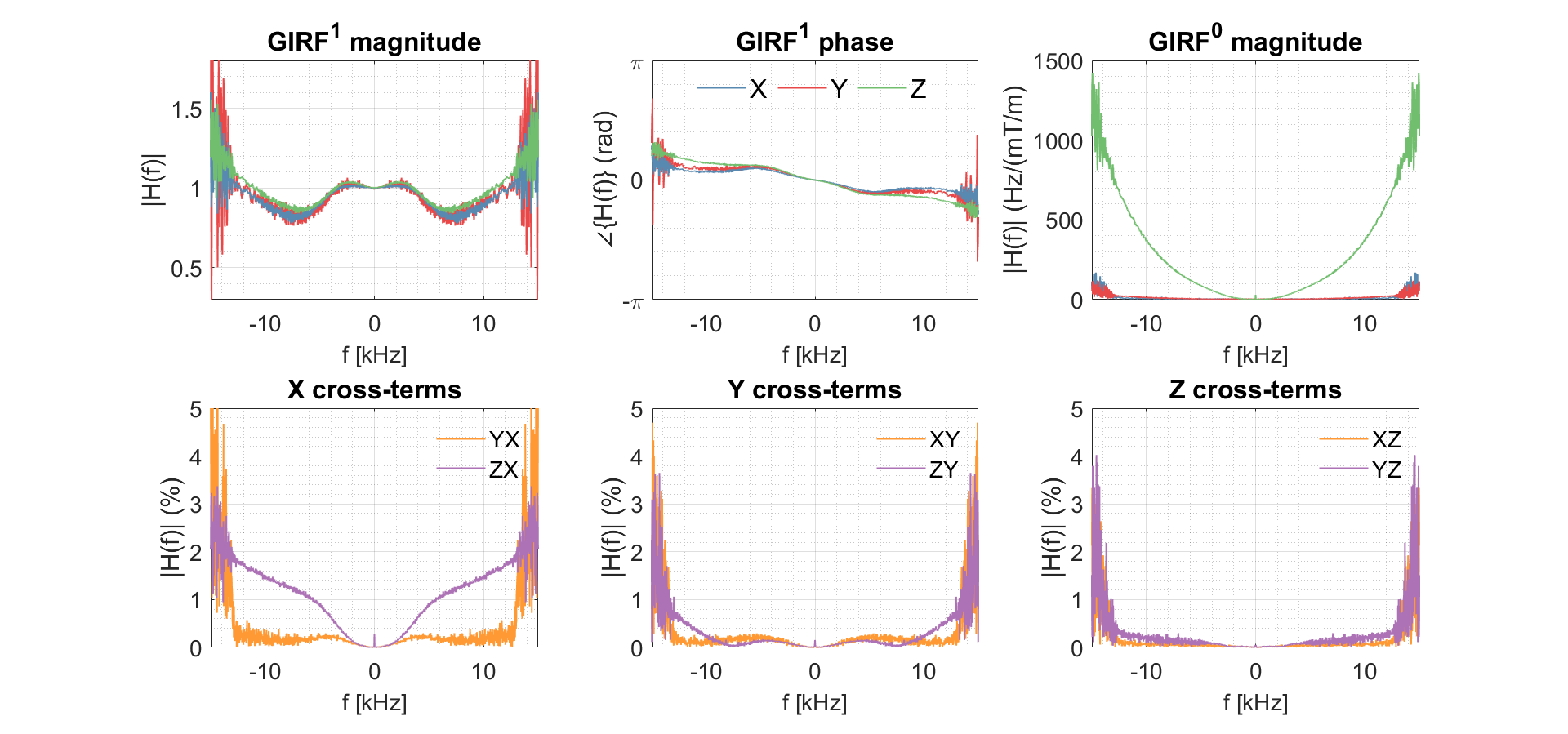
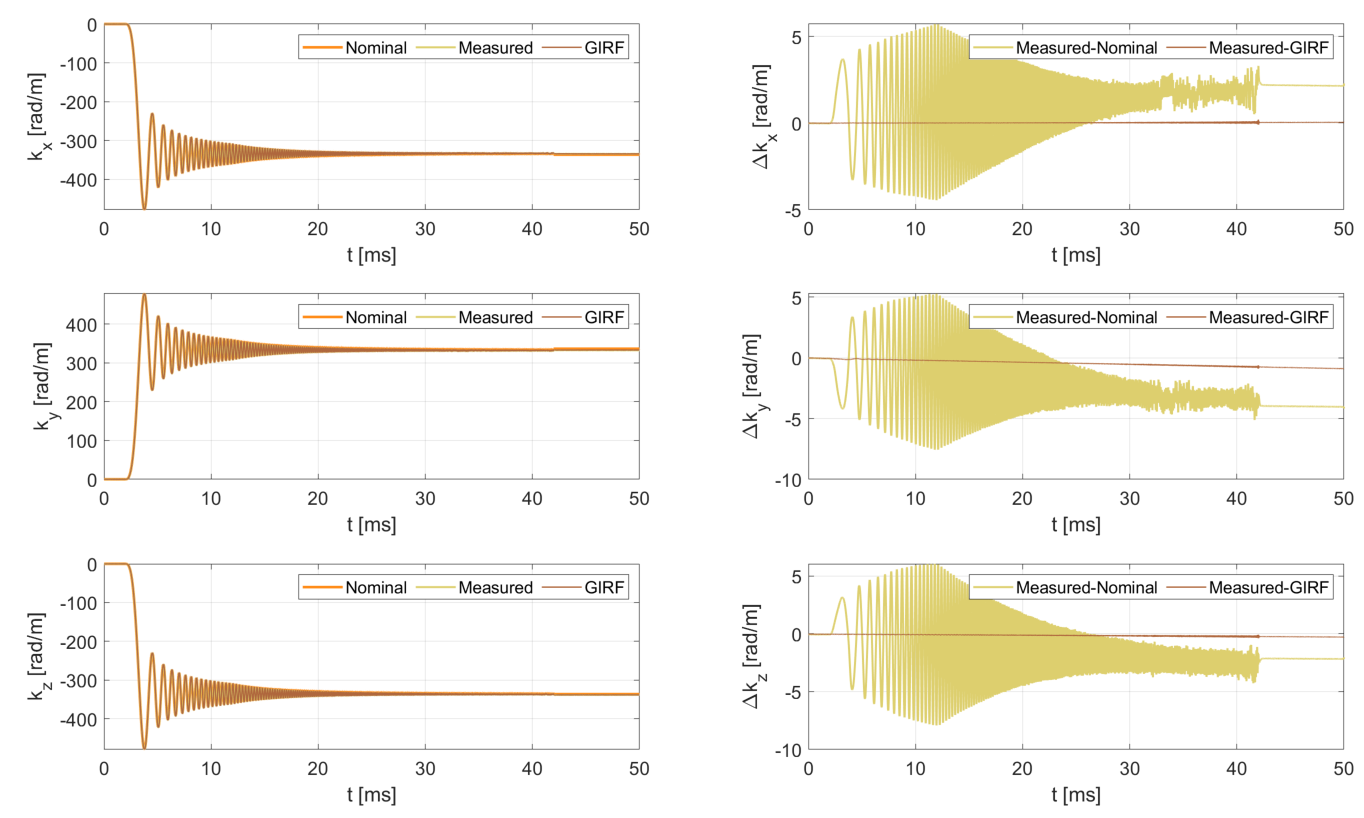
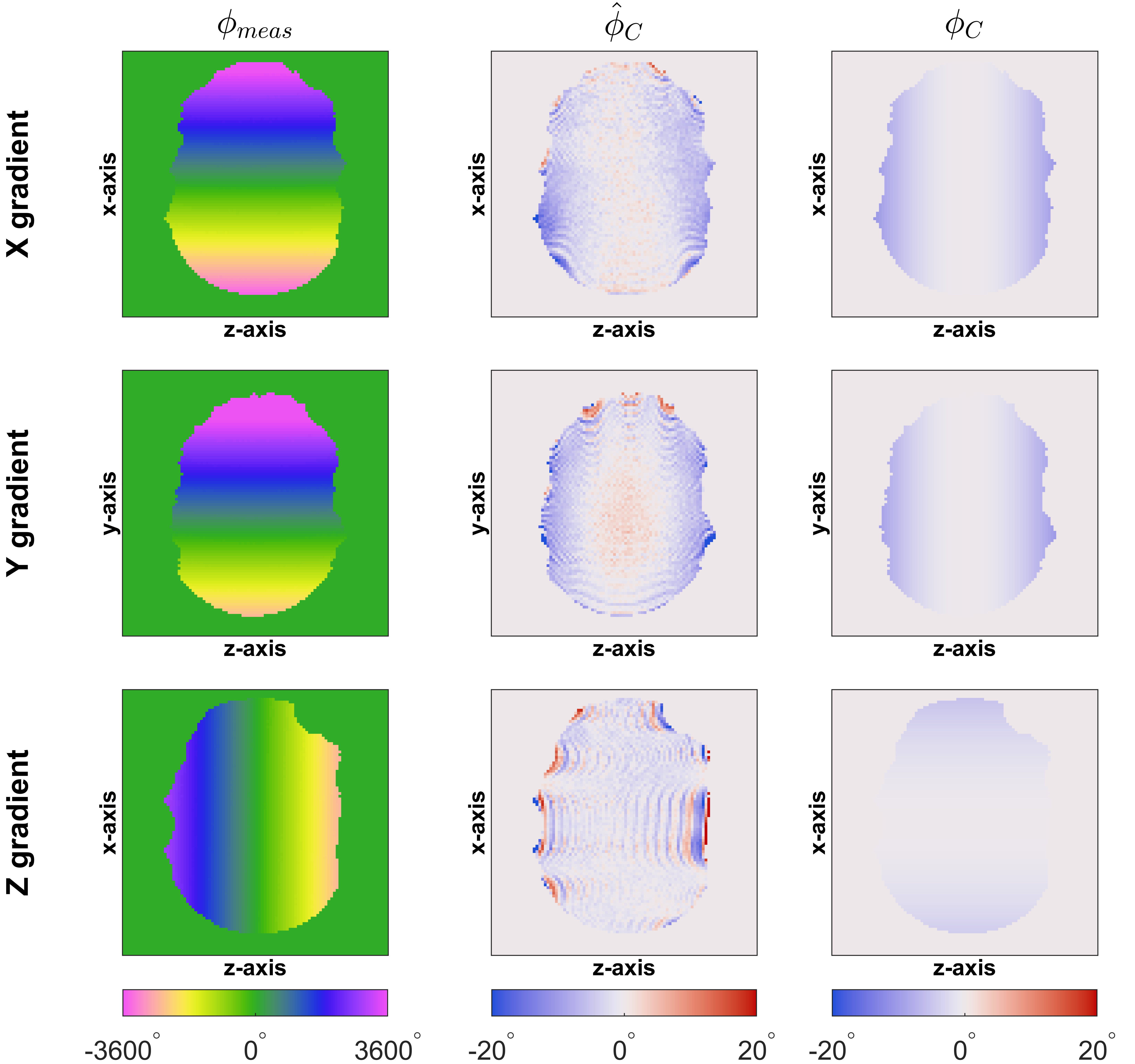
Figure 2 shows a full set of GIRF terms. Zeroth-order terms are generally small with the largest being in the z-direction. First-order self-terms are similar to one another and an "m-shaped" variation with frequency is observed. Cross-terms are also small with the largest effect seen on the x-axis when applying a gradient along the z-direction. Figure 3 demonstrates that GIRF estimation is successful; trajectory residuals are almost zero when applying the measured GIRF to $$$\mathrm{\mathbf{g_{nom}}}$$$.

Figure 4 shows $$$\phi_{\mathrm{meas}}$$$ in all three orientations and compares the estimated $$$\hat\phi_{\mathrm{C}}$$$ to the analytical $$$\phi_{\mathrm{C}}$$$. The concomitant phase effects are far smaller than the measured total phase. Broad agreement is apparent for the x-gradient and y-gradient; the phase variation along the z-axis is replicated in $$$\hat\phi_{\mathrm{C}}$$$ and $$$\phi_{\mathrm{C}}$$$. Differences are apparent for the z-gradient due to undiagnosed imaging artefacts, potentially due to susceptibility effects. Lee et al.⁹ use the system GIRF to predict Maxwell terms for phase correction in image reconstruction. Essentially their estimate of the Maxwell phase is the same as $$$\phi_{\mathrm{C}}$$$ shown here. We provide experimental measurement $$$\hat\phi_{\mathrm{C}}$$$ which matches this prediction well, suggesting that the MaxGIRF method (i.e. use of a linear GIRF plus analytically calculated Maxwell and measured B₀ terms) is a good model for total phase variation in a lower field MR system.

Conclusions

The developed sequence and pipeline have shown potential for gradient characterization and Maxwell field phase estimation at low field from the same dataset. Going forward, these measurements can be used to improve the image quality at 0.55T, especially for methods that are prone to gradient imperfections.

Acknowledgements

Daniel West and David Leitão contributed equally to this work. The research was funded/supported by core funding from the Wellcome/EPSRC Centre for Medical Engineering [WT203148/Z/16/Z] and by the National Institute for Health Research (NIHR) Biomedical Research Centre based at Guy's and St Thomas' NHS Foundation Trust and King's College London and/or the NIHR Clinical Research Facility. The views expressed are those of the author(s) and not necessarily those of the NHS, the NIHR or the Department of Health and Social Care.

References

1. Barmet C, De Zanche N, Pruessmann KP. Spatiotemporal magnetic field monitoring for MR. Magn. Reson. Med. 2008;60:187–197 doi: 10.1002/mrm.21603.

2. De Zanche N, Barmet C, Nordmeyer-Massner JA, Pruessmann KP. NMR Probes for measuring magnetic fields and field dynamics in MR systems. Magn. Reson. Med. 2008;60:176–186 doi: 10.1002/mrm.21624.

3. Addy NO, Wu HH, Nishimura DG. Simple method for MR gradient system characterization and k-space trajectory estimation. Magn. Reson. Med. 2012;68:120–129 doi: 10.1002/mrm.23217.

4. Vannesjo SJ, Haeberlin M, Kasper L, et al. Gradient system characterization by impulse response measurements with a dynamic field camera. Magn. Reson. Med. 2013;69:583–593 doi: 10.1002/mrm.24263.

5. Duyn JH, Yang Y, Frank JA, Veen JW Van Der. Simple Correction Method for k-Space Trajectory Deviations in MRI. J. Magn. Reson. 1998;153:150–153.

6. Brodsky EK, Klaers JL, Samsonov AA, Kijowski R, Block WF. Rapid measurement and correction of phase errors from B0 eddy currents: Impact on image quality for non-cartesian imaging. Magn. Reson. Med. 2013;69:509–515 doi: 10.1002/mrm.24264.

7. Campbell-Washburn AE, Xue H, Lederman RJ, Faranesh AZ, Hansen MS. Real-time distortion correction of spiral and echo planar images using the gradient system impulse response function. Magn. Reson. Med. 2016;75:2278–2285 doi: 10.1002/mrm.25788.

8. Rahmer J, Mazurkewitz P, Börnert P, Nielsen T. Cross Term and Higher Order Gradient Impulse Response Function Characterization using a Phantom-based Measurement. In: Proc. Intl. Soc. Mag. Reson. Med. 26. ; 2018.

9. Lee NG, Ramasawmy R, Lim Y, Campbell‐Washburn AE, Nayak KS. MaxGIRF: Image reconstruction incorporating concomitant field and gradient impulse response function effects. Magn. Reson. Med. 2022:1–20 doi: 10.1002/mrm.29232.

10. Papadakis NG, Wilkinson AA, Carpenter TA, Hall LD. A general method for measurement of the time integral of variant magnetic field gradients: Application to 2D spiral imaging. Magn. Reson. Imaging 1997;15:567–578 doi: 10.1016/S0730-725X(97)00014-3.

Figures

Figure 1: Sequence diagram of a single-slice acquisition designed to have two phase-encoding gradients, which enables measurement of the magnetization response to a test waveform. This example shows a variable amplitude chirp test waveform played out on both phase-encoding axes, although data was also acquired with the waveform on each axis individually and on neither axis (for the reference scan).

Figure 2: Measurement of all GIRF terms: first-order self-terms are shown on the top row for all three directions, alongside corresponding zeroth-order terms. Cross-terms are on the bottom row; the first character in the legend denotes the physical axis along which the variable amplitude chirp gradient is played and the second denotes the measurement axis.

Figure 3: Trajectories in each direction corresponding to the nominal ($$$\mathbf{\mathrm{g_{nom}}}$$$), measured ($$$\mathbf{\mathrm{g}}$$$) and GIRF-corrected gradient waveforms. Residuals are shown on the zoomed right-hand side plot before (yellow) and after (brown) GIRF correction.

Figure 4: Comparison of the estimated Maxwell phase with respect to its analytic equivalent. The overall measured phase is plotted on the left-hand side as a reference. All displayed phases are from TE = 50ms.

Proc. Intl. Soc. Mag. Reson. Med. 31 (2023)

4570

DOI: https://doi.org/10.58530/2023/4570