Synopsis

Keywords: Gradients, Gradients, concomitant field

We show that concomitant field-induced phase in phase-contrast imaging allows measurement of the transverse (x,y) components of the magnetic field generated by a gradient coil. Combined with conventional B₀ mapping which gives the z-component, the method permits experimental determination of the full three-dimensional vector magnetic field of a gradient coil. We demonstrate the method on a high-performance head gradient (MAGNUS) system and discuss its application to concomitant-field artifact correction based on one-time calibration.

Introduction

In MRI, concomitant field refers to the transverse (B_x, B_y) components of the magnetic field that necessarily accompany spatial variation of the z-directional magnetic field (B_z) generated by the gradient coils during image encoding. The concomitant field has been most extensively studied for its effects on image artifacts [1], but it also contributes to peripheral nerve stimulation (PNS) [2] and implant heating [3]. Despite its importance, direct measurement of B_x, B_y fields is not easy because traditional field mapping methods measure the total magnetic field which is dominated by B_z. Here we show that a balanced bipolar gradient pulse can encode the transverse magnetic field into the image phase, and strategic acquisition of such data followed by azimuthal symmetry-based post-processing allows us to map out the full vector magnetic field of a gradient coil in 3D space.

Theory

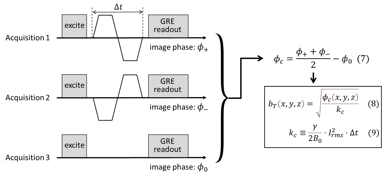
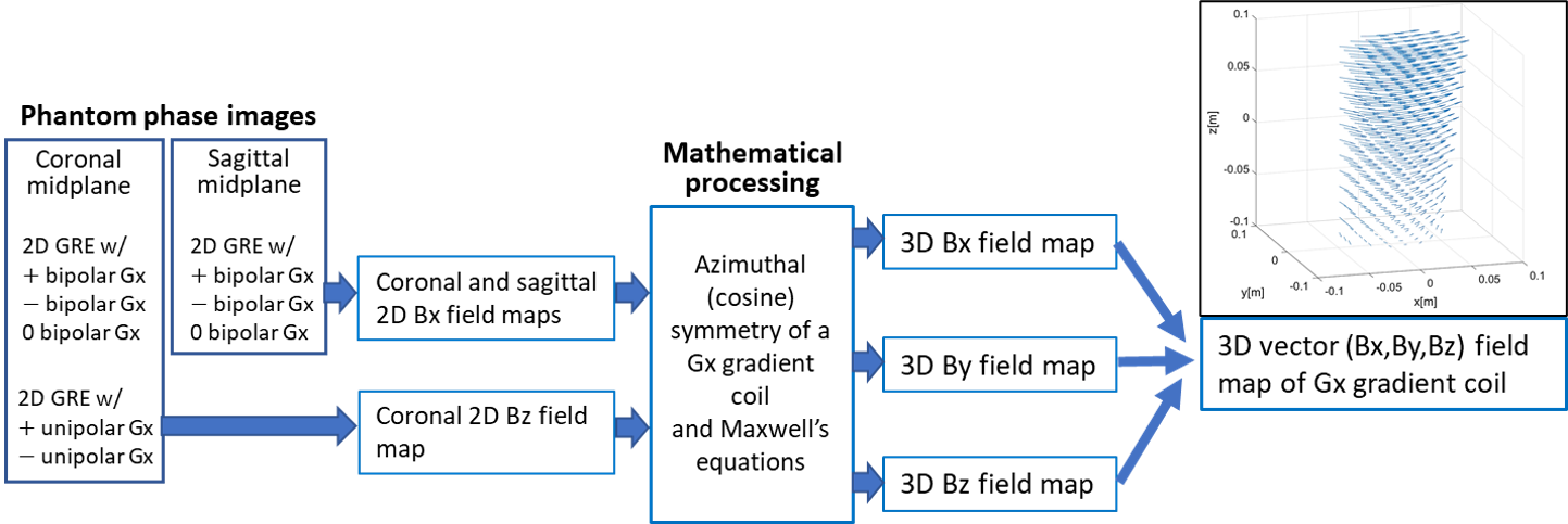
Isolation of transverse field phase. Consider a gradient coil which produces an x-directional field B_T as well as a z-directional one B_g at a particular voxel. The total magnetic field vector (B_tot) at the voxel consists of the gradient field vector, main magnetic field B₀, static off-resonance field B_s, and the eddy current field B_e (Eq. (1)). The magnitude of B_tot can be expressed as Eq. (2) where we retained terms up to the second order in the small parameter δ. Importantly, in Eq. (2) the longitudinal (B_z,all) and transverse (B_T) field terms are separated. Eq. (3) shows the instantaneous Larmor frequency. When a bipolar gradient pulse is applied for time Δt, the voxel accrues phase due to B_s, B_e, B_T (Eq. (4)). The B_e term reverses sign if the opposite-polarity pulse is applied (Eq. (5)), and the B_s term is isolated if the pulse is zeroed (Eq. (6)). The three phases φ₊, φ_-, φ₀ can be combined to compute φ_c (Eq. (7), Fig. 2) which gives the desired magnitude of B_T (Eq. (8)).
3D vector field calculation. The azimuthal (m=1) symmetry of a transverse gradient coil implies that two measurements of B_T, on the coronal and sagittal midplanes, are sufficient to calculate the transverse magnetic field anywhere in a cylindrical volume. When this information is combined with the longitudinal field B_z that can be measured by phase induced by an unbalanced (unipolar) gradient pulse, we can reconstruct a 3D vector field map of the gradient coil (Fig. 3). For an axi-symmetric (m=0) longitudinal gradient coil (Gz), B_T measurement on one (e.g. coronal) plane suffices to enable 3D reconstruction.

Experimental Methods

All experiments were performed with a high-performance head gradient coil (MAGNUS)[4] inserted in a whole-body 3T magnet, using a cylindrical phantom and a volume T/R coil. Figure 2 shows the schematic of the modified 2D gradient echo-based phase-contrast imaging sequence used to produce the three phase images. Representative scan parameters are TR/TE/Δt = 200/8.3/4.4 ms; FOV/ slice thickness/ isotropic pixel size = 260/5/1.35 mm. Real-time concomitant field correction [5] was disabled. Two more phase images were obtained for B_z mapping. The phase images were processed following the workflow of Fig. 3. The experiment was repeated for x, y, z gradient coils. The resulting vector field maps were compared with the gradient coil's electromagnetic (EM) design.

Results

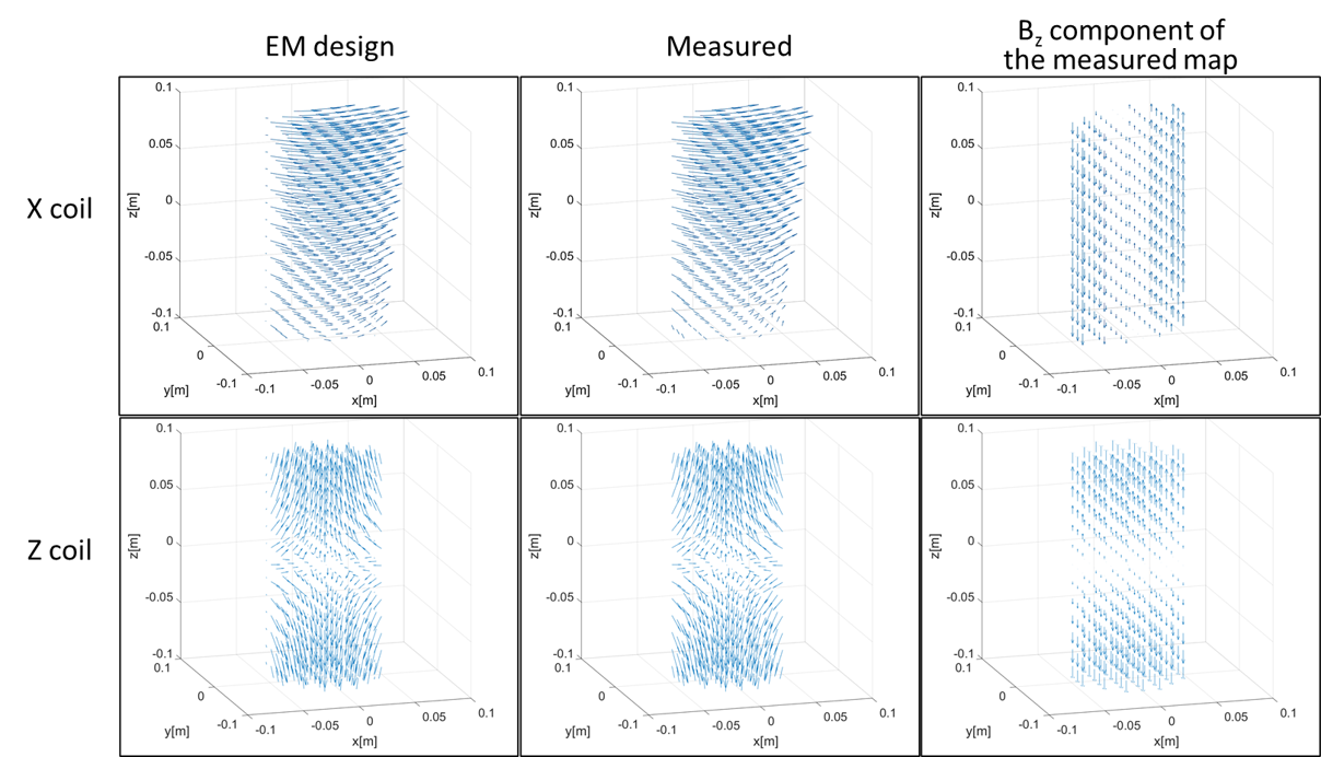
The middle column of Fig. 4 shows the measured vector field maps of the x- and z-gradient coils. The maps visually agree well with the EM-design field maps shown on the left column. Our data enable direct visualization of the strong concomitant fields of an asymmetric (x) gradient coil, which is evident when compared with the z-component-only map (right column). The field maps for the y-coil were similar to the x-coil, rotated by 90 degrees in the xy-plane. Quantitative comparison showed that the measurement error (compared to the EM design) was less than ~5% within 5 cm from the isocenter, but gradually increased with distance (not shown). The discrepancy is possibly due to vibration-induced phase that is quadratic to the bipolar pulse amplitude, which is not cancelled by phase combination of Eq. (7).

Discussions and Conclusion

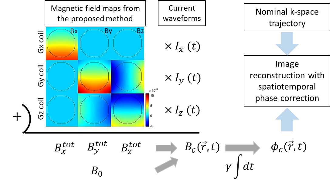
Full knowledge of the vector magnetic field generated by the gradient coils allows one to model spatio-temporal evolution of the total encoding magnetic field during imaging. This enables prediction of the concomitant-field-induced phase evolution at every voxel, which can inform prospective correction mechanisms (such as gradient pre-emphasis) or artifact correction in post-processing (Fig. 5). The proposed method can also be used to obtain full vector magnetic field data for electric field calculation, for the purpose of PNS simulation or eddy current assessment, without resorting to gradient coil EM design.
To date, experimental concomitant field measurement has fallen under two categories: (i) low spatial-order parameter fitting under linear gradient assumption [6], and (ii) dynamic Larmor frequency measurement by an NMR probe array for individual sequences [7]. The proposed method is advantageous in that it is applicable to nonlinear gradients and allows sequence-independent calibration. In conclusion, we have demonstrated an experimental method to measure the three-dimensional vector magnetic field produced by a gradient coil. The experimental data showed good agreement with the EM design and hold promise for data-driven correction of concomitant field artifacts in high-performance gradient systems.

Acknowledgements

This work was supported by CDMRP W81XWH-16-2-0054. This presentation does not necessarily represent the official views of the funding agency.