4568
Modelling the gradient system as linear and time-invariant: Do the assumptions break down at higher field strength?1Siemens Healthineers International AG, Zurich, Switzerland, 2Swiss Center for Musculoskeletal Imaging (SCMI), Balgrist Campus, Zurich, Switzerland, 3Advanced Clinical Imaging Technology (ACIT), Siemens Healthineers International AG, Lausanne, Switzerland, 4Department of Diagnostic and Interventional Radiology, University Hospital Würzburg, Würzburg, Germany
Synopsis
Keywords: System Imperfections: Measurement & Correction, Gradients, GIRF, GSTF
The gradient system transfer function (GSTF) is a broadly used model to characterize the gradient chain and correct for imperfections e.g. in non-Cartestian sampling trajectories. The model assumes linearity and time-invariance (LTI) of the system. In this work, we indirectly examine the LTI compliance across two different field strengths by comparing different GSTFs based on varying subsets of input gradient shapes for the model computation. Overall, only small changes in the GSTF were observed upon adding different input gradients for the system characterization. However, the differences were more pronounced at 7T compared to 3T.Introduction
For non-Cartesian MRI trajectories like spiral or radial, gradient waveform corrections are often required to ensure good image quality. The gradient impulse response function (GIRF)1 or its Fourier transform, the gradient system transfer function (GSTF), is a broadly used model to characterize the gradient system, assuming linearity and time-invariance (LTI). However, certain properties, e.g. non-linear effects of gradient amplifiers2 or heating effects3, might violate those assumptions.Efforts to incorporate non-linearities in a GSTF-based system characterization have been made by modelling the temperature dependence3–5, or by using the amplifier’s output currents as input for the LTI model2.
In this work, we indirectly examine the LTI compliance of the gradient chain across two different field strengths by comparing different GSTFs based on varying subsets of input gradient shapes for the model computation.
Methods
We acquired three subsets of gradient pulses (small triangles, large triangles, and a trapezoidal gradient) to estimate the GSTF. They were all acquired with research application sequences using the thin slice method6 as described earlier7. The measurements were performed at 3T and 7T (MAGNETOM Prisma and Terra, Siemens Healthcare, Erlangen, Germany) using a spherical phantom in the head coil. Table 1 provides measurement details.Three GSTFs were determined, each based on different subsets of the acquired gradient pulses. GSTF1 only relies on the small triangle data, GSTF2 encompassed the small and large triangles, and GSTF3 combined all available gradient shapes, i.e. small and large triangles, and the trapezoidal gradient. We examined the accuracy of the different GSTF models by comparing their predictions of the trapezoidal gradient evolution to the actual measurement.
For a perfect LTI system, all GSTFs would be identical. To compare them quantitatively, the RMSE to GSTF3 (full model) was calculated in the range from -5kHz to 5kHz for both phase and magnitude on all three physical gradient axes.
Results
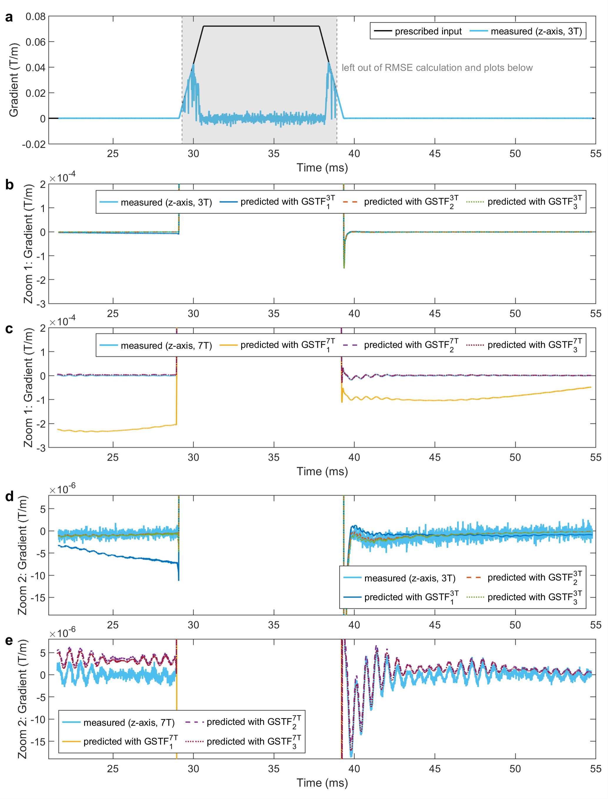
Figure 1 displays the gradient system transfer functions’ (GSTF1-3) magnitude of the z-axis measured at 3T (left) and 7T (right) in the top row. Subplots (c)-(f) show the magnitude difference of GSTF1 and GSTF2 to GSTF3 in two frequency ranges, namely -10 kHz to 10 kHz (middle) and -5 kHz to 5kHz (bottom). Seeing that the difference between GSTF1 and GSTF3 starts to be noise-dominated at approximately ±6 kHz (Figure 1(d)), we limited the range for the quantitative comparison to ±5 kHz.Figure 2 depicts the measured and predicted gradient responses for all three different GSTFs for the trapezoidal test gradient (a). Subplots (b)–(e) show zoomed-in versions to highlight differences between the curves.
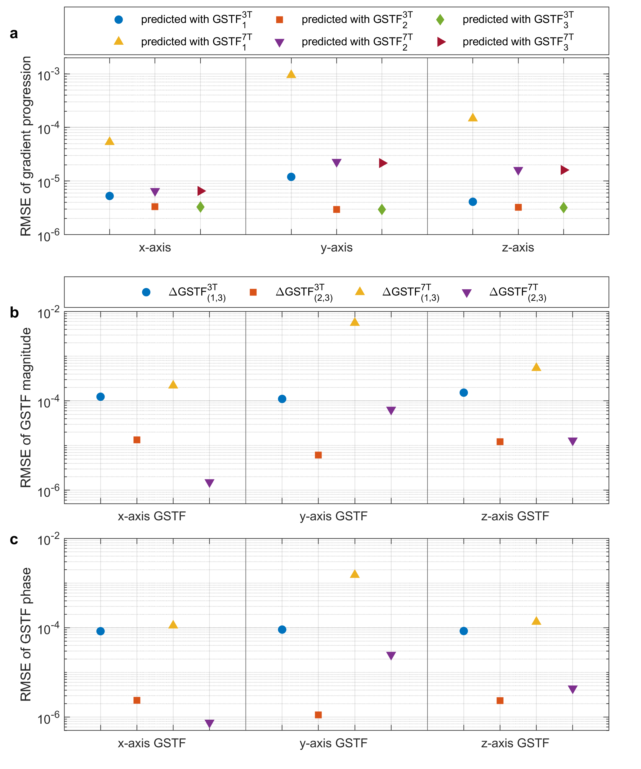
Figure 3 quantitatively compares the RMSE between measured and predicted evolutions of the trapezoidal test gradient (a), as well as between different GSTFs (in ±5kHz range) on both 3T (Prisma) and 7T (Terra). GSTF3 is used as baseline model in (b) and (c).
Discussion
All three GSTFs predict the gradient time course reasonably well for both 3T and 7T. However, small deviations between the measured and predicted gradient shapes can be observed in Figure 2(b)–(e). The change of gradient predictions between different GSTF models is larger on 7T compared to 3T for the given test case and the GSTF based on the full set of calibration gradients, GSTF3, predicts the measured time courses with the lowest RMSE (Figure 3(a)). For the quantitative model comparison (Figure 3 (b)-(c)), GSTF3 was therefore chosen as reference model. This direct model comparison is independent of a chosen test gradient and should lead to a more general conclusion despite the lack of a ground truth. On all three physical gradient axes, and on both scanners, the RMSE between GSTF1 and GSTF3 is larger than the RMSE between GSTF2 and GSTF3. Furthermore, the RMSE of each GSTF comparison on the 7T system exceeds the RMSE of the respective comparison on the 3T system, except for the RMSE between GSTF2 and GSTF3 on the physical x-axis. It therefore seems that the LTI assumptions hold better for 3T than 7T. Potential explanations for a “less-LTI-like” behavior at higher field strength might be increased mechano-magnetic coupling, or transient oscillations. However, it is important to note that, besides the difference in field strength, other system-dependent factors, e.g. hardware components, could also influence the linearity and time-invariance of the gradient chain.A limitation of this work is that the effect of different GSTFs on image quality of non-Cartesian trajectories was not examined. We assume that small changes in gradient predictions might not have a noticeable impact on image quality in many cases. Demonstrated successful applications of GSTF models to non-Cartesian imaging at 7T in the literature7,8 support this hypothesis. Additionally, this study was limited to only two field strengths (3T and 7T) and one test gradient shape (trapezoid). Further investigations, e.g. at both lower and even higher field strength, might give more insights on the question if and when deviations from the LTI assumptions need to be accounted for.
Conclusion
We examined the LTI compliance of the gradient system across two different field strengths. Overall, only small changes in the GSTF were observed upon adding different input gradients for the system characterization. However, the differences were more pronounced on the 7T scanner than at 3T.Acknowledgements
No acknowledgement found.References
1. Vannesjo, S. J. et al. Image reconstruction using a gradient impulse response model for trajectory prediction. Magn. Reson. Med. 76, 45–58 (2016).
2. Rahmer, J., Schmale, I., Mazurkewitz, P., Lips, O. & Börnert, P. Non-Cartesian k-space trajectory calculation based on concurrent reading of the gradient amplifiers’ output currents. Magn. Reson. Med. 3060–3070 (2021). doi:10.1002/mrm.28725
3. Stich, M. et al. The temperature dependence of gradient system response characteristics. Magn. Reson. Med. 83, 1519–1527 (2020).
4. Wilm, B. J., Dietrich, B. E., Reber, J., Johanna Vannesjo, S. & Pruessmann, K. P. Gradient Response Harvesting for Continuous System Characterization during MR Sequences. IEEE Trans. Med. Imaging 39, 806–815 (2020).
5. Nussbaum, J., Dietrich, B. E., Wilm, B. J. & Pruessmann, K. P. Thermal variation in gradient response: measurement and modeling. Magn. Reson. Med. 87, 2224–2238 (2022).
6. Duyn, J. H., Yang, Y., Frank, J. A. & Van Der Veen, J. W. COMMUNICATIONS Simple Correction Method for k-Space Trajectory Deviations in MRI The new method measures the actual k-space trajectories. J. Magn. Reson. 132, 150–153 (1998).
7. Vannesjo, S. J. et al. Gradient and shim pre-emphasis by inversion of a linear time-invariant system model. Magn. Reson. Med. 78, 1607–1622 (2017).
8. Graedel, N. N. et al. Feasibility of spiral fMRI based on an LTI gradient model. Neuroimage 245, 118674 (2021).
Figures
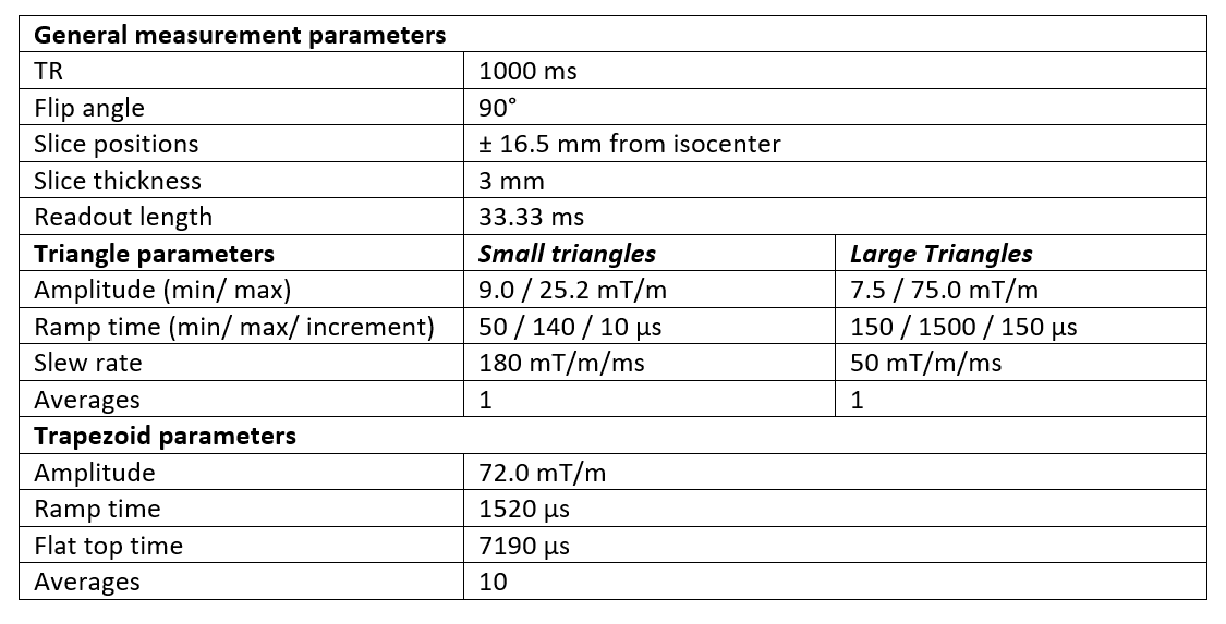
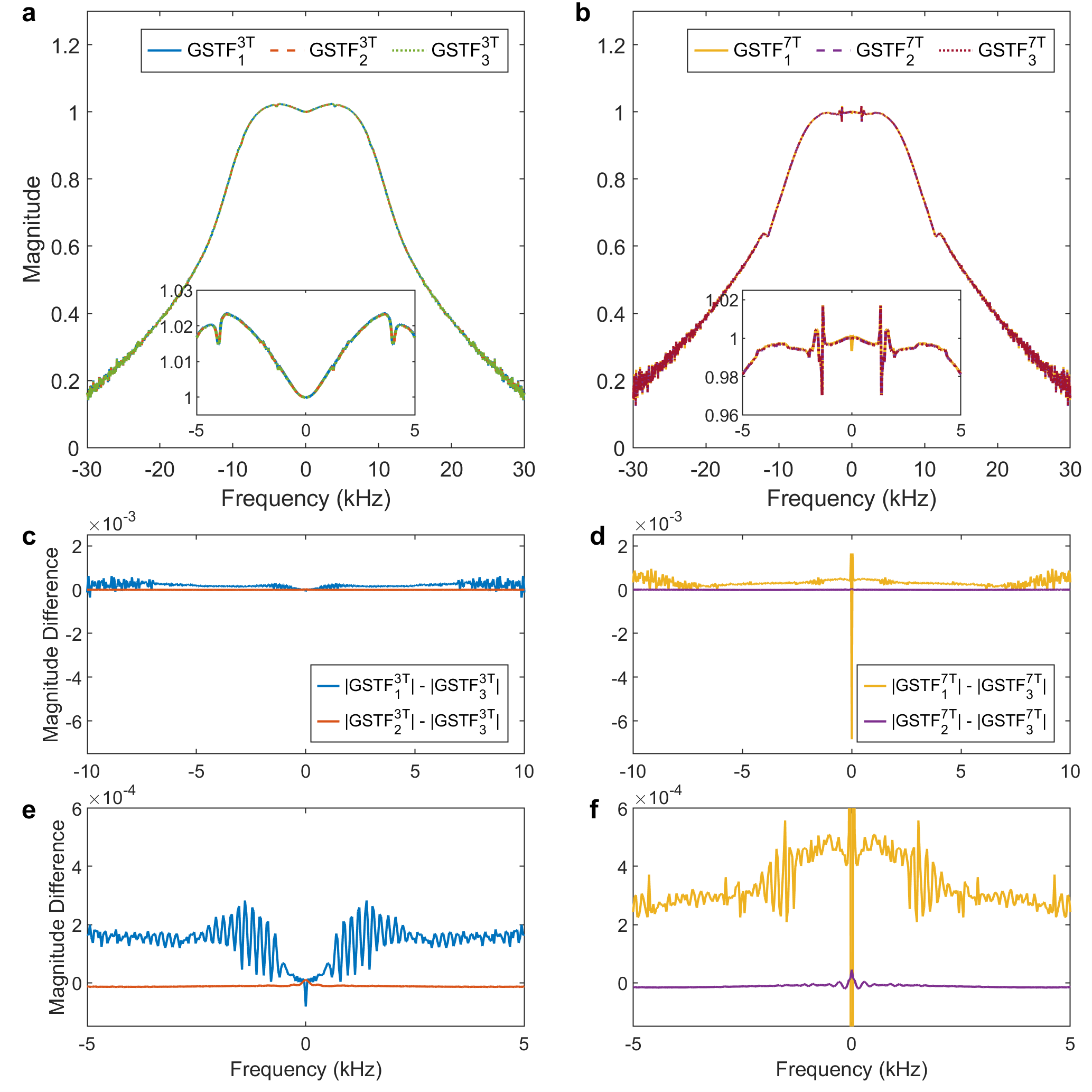
Figure 1. (a,b) Magnitude of GSTFs of the z- axis for both 3T (Prisma, a) and 7T (Terra, b), calculated with different subsets of gradient pulses. (c,d) Magnitude differences in the frequency range from -10 kHz to 10 kHz. (e,f) Zoom into the range from -5 kHz to 5 kHz, which was used for the RMSE calculation.