4475
RECOMPOSE – Reproducing DECOMPOSE Using Susceptibility Maps Acquired for Clinical Research1Medical Physics and Biomedical Engineering, University College London, London, United Kingdom, 2Electrical Engineering and Computer Sciences, University of California, Berkeley, Berkeley, CA, United States, 3Helen Wills Neuroscience Institute, University of California, Berkeley, Berkeley, CA, United States
Synopsis
Keywords: Susceptibility, Quantitative Susceptibility mapping
Here, we reproduced the results of the DECOMPOSE susceptibility separation model using new $$$T_2^*$$$-weighted data independently acquired using three clinically applicable sequences and processed with different QSM pipelines. This allowed us to investigate the sensitivity of DECOMPOSE to various dipole inversion algorithms. Good susceptibility source separation results were achieved using a 5-echo GRE acquisition, but maps of diamagnetic and paramagnetic sources from a highly accelerated 5-echo EPI sequence were noisy. When the input susceptibility maps exhibited artefacts, these were exacerbated by DECOMPOSE. Care must be taken not to lose local structural information when using (highly) regularised input susceptibility maps.
Introduction
In quantitative susceptibility mapping (QSM) the goal is to reconstruct bulk magnetic susceptibility values in tissue from the measured phase. The susceptibility value in each voxel results from contributions from para- and diamagnetic molecules. DECOMPOSE, a method to separate these contributions based on fitting a three-compartment model to multi-echo gradient recalled echo (GRE) data, was introduced at ISMRM 20211. It was then validated using a phantom, and successfully applied to high signal-to-noise-ratio (SNR) 16-echo GRE data of in vivo acquisitions2. DECOMPOSE has since been shown to benefit susceptibility based micro-structure detection3. This is the first application of DECOMPOSE using accelerated clinically applicable sequences and outside the group it was developed. Here, we aimed to reproduce the DECOMPOSE results using new data, acquired using shorter, more clinically applicable acquisitions with fewer echoes. Our goal was to test DECOMPOSE's ability to separate susceptibility sources in these lower signal-to-noise datasets with minimal number of echoes, to test its sensitivity to different QSM reconstruction algorithms used in the pre-processing pipeline, and to reproduce the original results using different acquisition and processing approaches.Methods
We applied DECOMPOSE in three different datasets acquired in healthy volunteers as part of previous studies4-6: 1. a conventional 5-echo 3D-GRE, 2. a 7-echo multi-parametric mapping (MPM) sequence with short echo times and only phase differences reconstructed7, and 3. a highly accelerated (low SNR) 5-echo 2D echo planar imaging (EPI) sequence. See Figure 1 for detailed sequence parameters. The 3D-GRE sequence (optimized for clinical QSM8-10) was used to reproduce the original DECOMPOSE results with just 5 echoes (the theoretical limit of the model). Sequences 2. and 3. were chosen as MPM and EPI are often encountered in clinical research studies for quantitative parameters or functional MRI, respectively.Single-echo QSM for all echoes in all three datasets were generated using the following QSM pipeline. A brain-mask was extracted using FSL BET11 (fractional intensity = 0.5). The phase images were unwrapped using a Laplacian method12,13 and background fields were removed using VSHARP ([18:-2:2] voxel kernel sizes, threshold of 0.05)14, followed by dipole inversion using a rapid two-step (RTS) approach with sparsity priors (d = 0.15, = 105, = 10, and stopping tolerance = 10-2)17. The processing pipeline can be found at: https://github.com/UCL-MedPhys-MRI/RECOMPOSE. In the EPI data slice-wise background field removal was applied15, followed by PDF (10-5 tolerance)16 to remove residual background fields.
The DECOMPOSE algorithm was run with default values: five iterations, diamagnetic susceptibility bounds of [-0.15, 0.05] and paramagnetic bounds of [-0.05,0.15] ppm. Several parameter variations were tried after observing inferior performance on the MPM dataset despite it having 7 echoes: DECOMPOSE was run with 10 iterations, then excluding the low phase-CNR first echo.
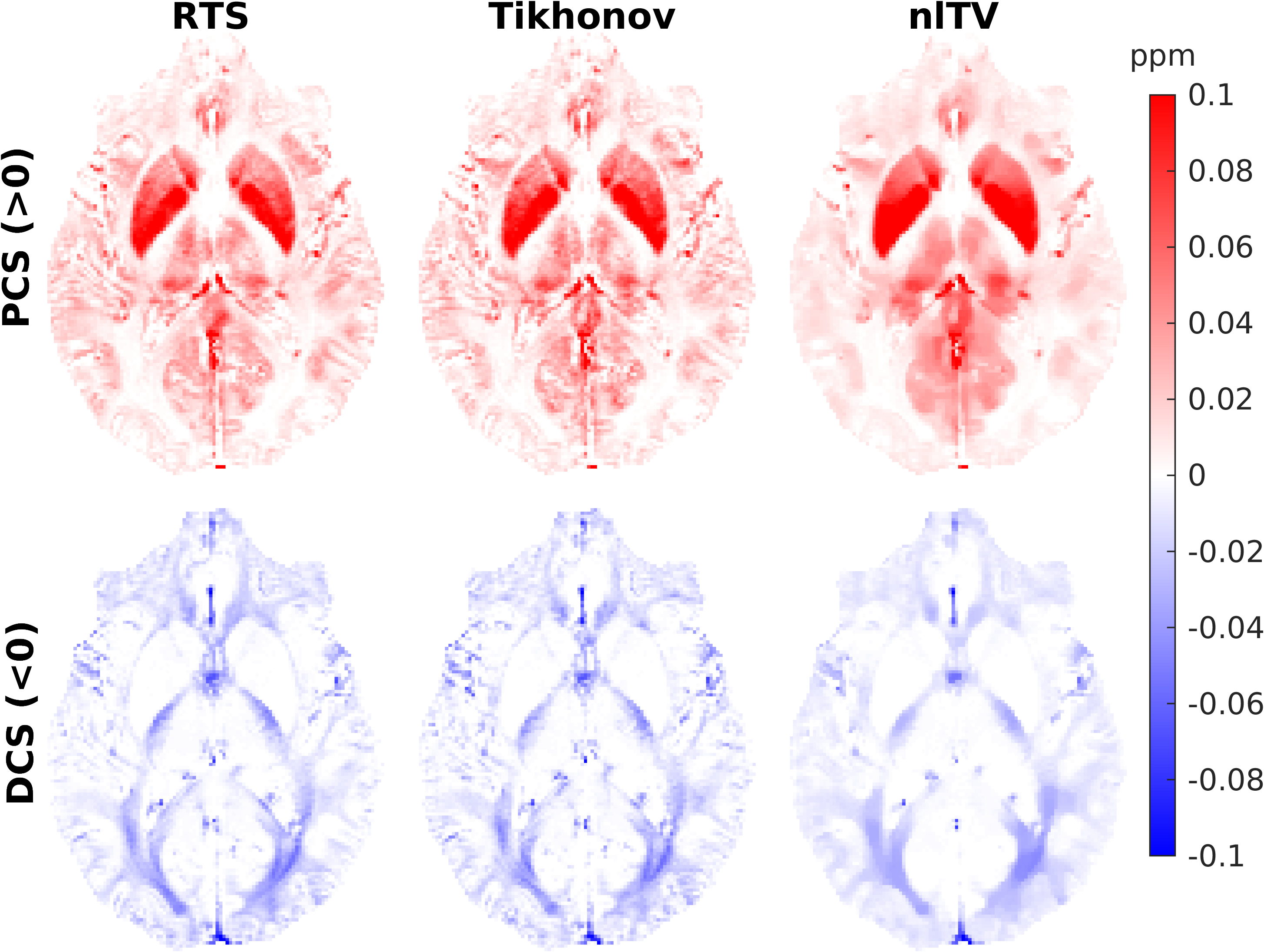
To investigate the sensitivity of DECOMPOSE to the QSM dipole inversion algorithm, DECOMPOSE was run on the 3D-GRE dataset with QSM pre-processing with the pipeline described above but using non-linear total variation (nlTV, l=0.001)18, and Tikhonov (a=0.01)19 regularizations with default regularisation weights. The decomposed maps were then compared with a susceptibility map from the (linearly combined) echoes, processed in the same way as the single echoes.
Results and Discussion
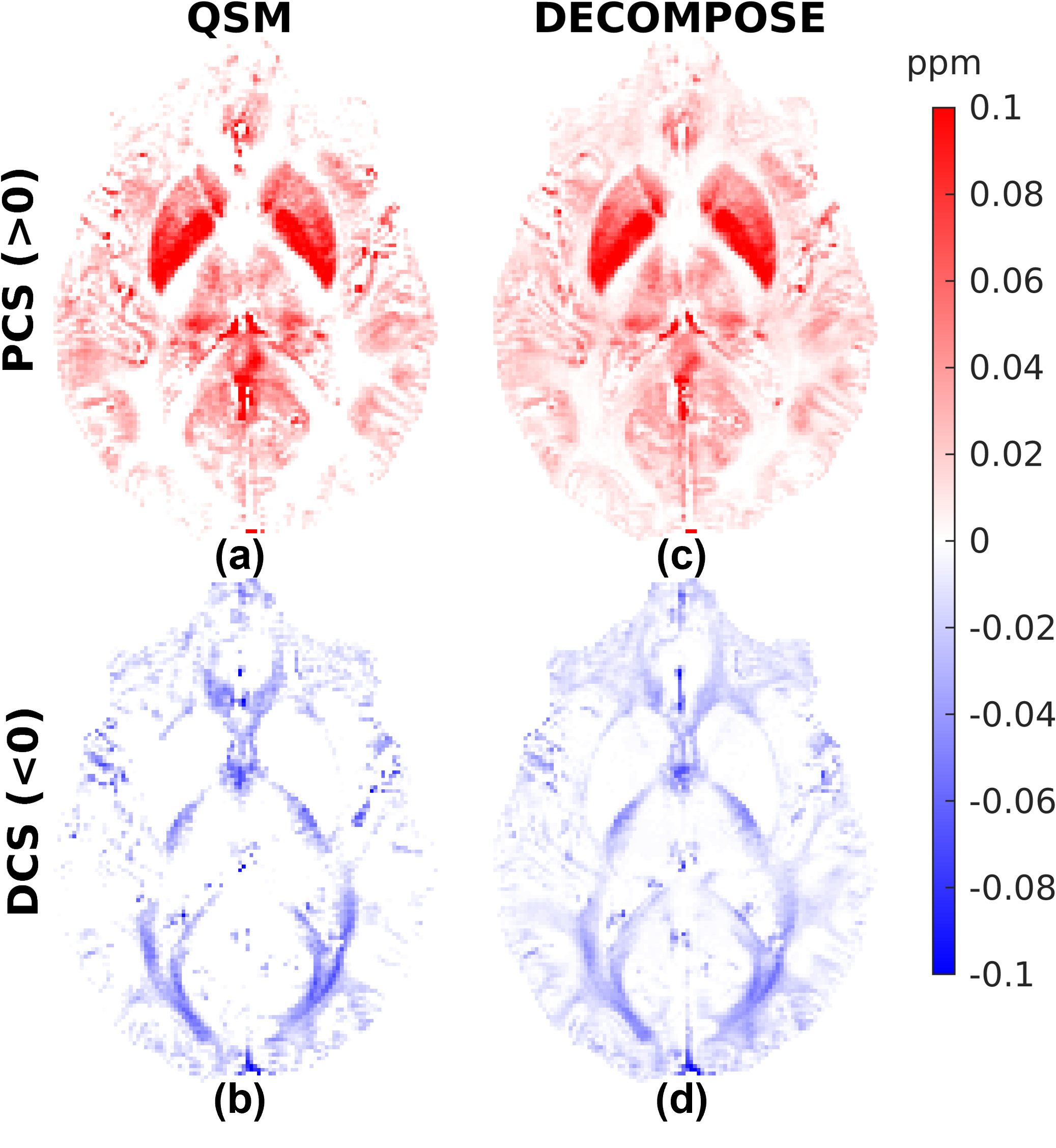
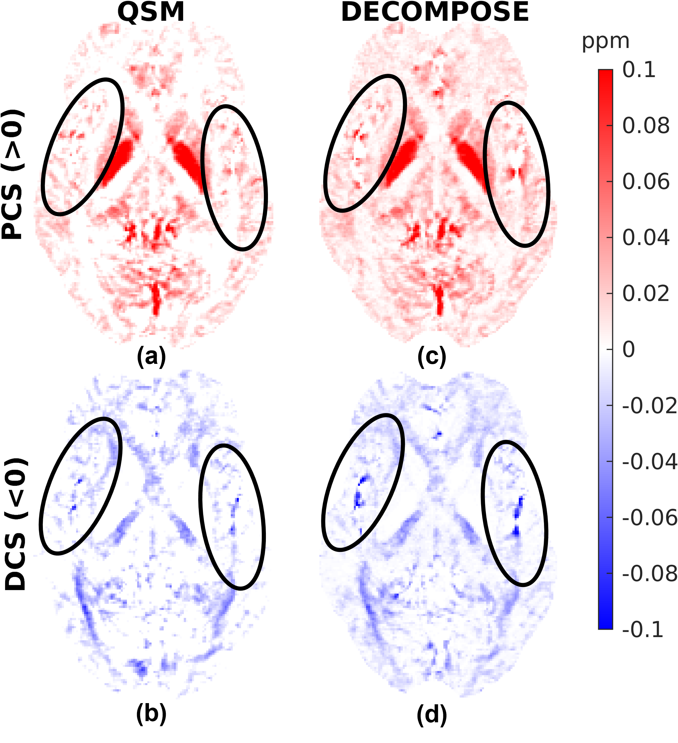
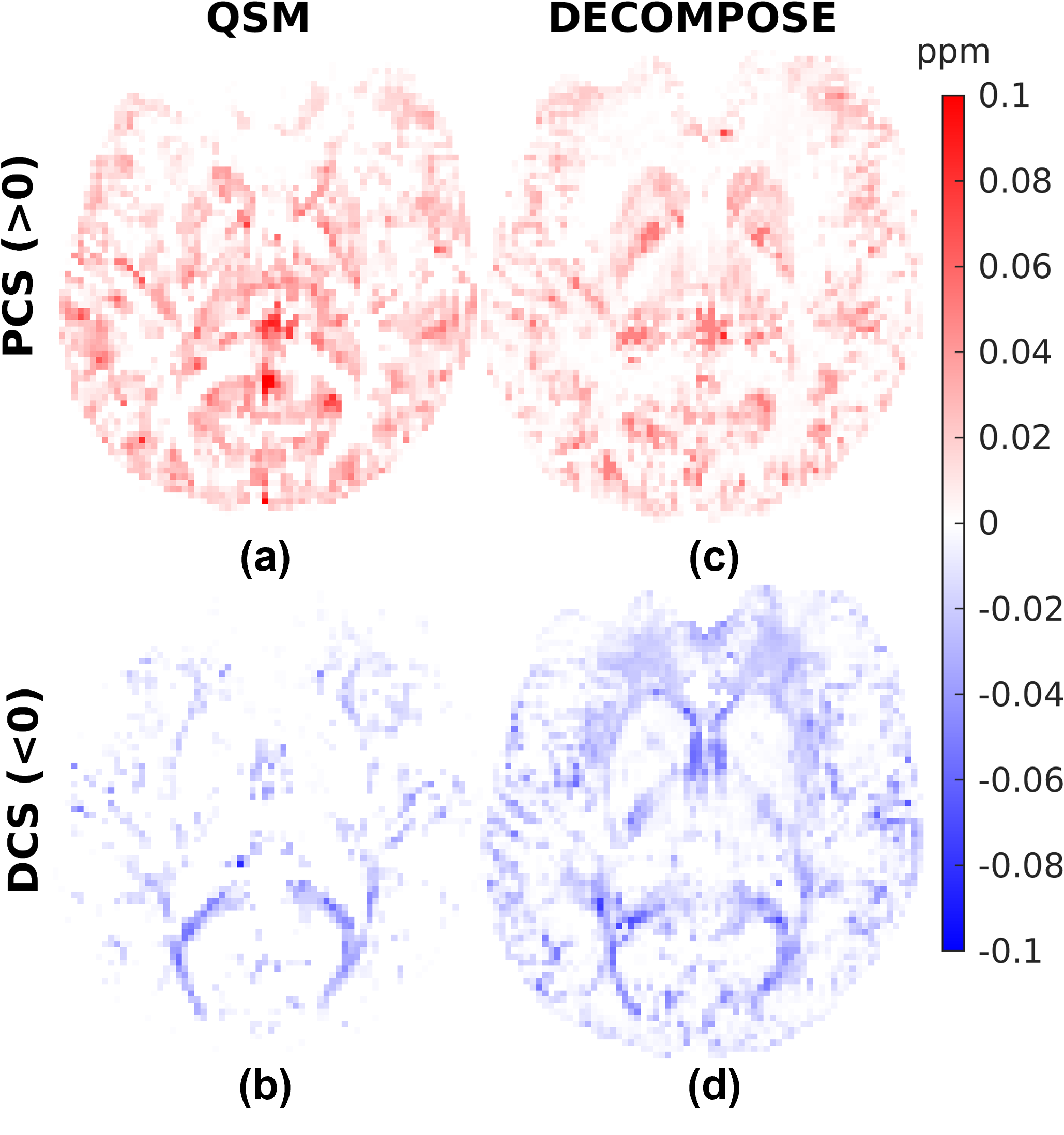
Figures 1, 2 and 3 show the DECOMPOSE maps from the GRE, MPM and EPI datasets, respectively. Figure 1 (c, d) show good agreement of the paramagnetic (PCS) and diamagnetic component of the susceptibility (DCS) with the component maps in the original publication2, with the DCS showing more extensive white matter regions than the thresholded QSM. Re-running DECOMPOSE on the MPM dataset with different parameters did not noticeably improve the resulting maps, and those presented here used the original parameters. The MPM DECOMPOSE maps in Figure 2 show artefacts from the QSM reconstruction. This dataset features very short echo spacing and only phase difference maps were reconstructed which seems to result in artefacts around vasculature (highlighted in the figure with black ovals) in the single echo maps, affecting the performance of DECOMPOSE.The EPI DECOMPOSE maps (Figure 3) appear noisier, possibly due to distortion and residual background fields, but perhaps resulting from the lower SNR, and larger echo spacing than the GRE and MPM. Figure 5 features a comparison between the 3D-GRE DECOMPOSE maps using three different QSM dipole inversion algorithms. It shows smoother para- and diamagnetic susceptibility maps for nlTV when compared to Tikhonov and RTS suggesting sub-voxel information is lost by regularisation in nlTV, which cannot be recovered by DECOMPOSE.
Conclusions
We reproduced DECOMPOSE maps similar to Chen2 with a shorter 5-echo GRE sequence and a different QSM processing pipeline. Using MPM and EPI sequences, the DECOMPOSE maps had noticeable artifacts and are of lower quality overall. These issues seem to be related primarily to the lower quality of input QSM maps, as the artefacts are also present in input QSM images (and not in the magnitude images). Additionally, our investigation into the sensitivity of DECOMPOSE to the dipole inversion method used shows that susceptibility map regularisation clearly affects the derived paramagnetic and diamagnetic susceptibility maps.The challenge of applying DECOMPOSE to faster sequences with fewer echo times highlights the importance of optimising the QSM pipeline: both minimising artefacts and preserving structural information when using DECOMPOSE.
Acknowledgements
Karin Shmueli and Patrick Fuchs were supported by European Research Council Consolidator Grant DiSCo MRI SFN 770939. Oliver Kiersnowski’s work was supported by the EPSRC-funded UCL Centre for Doctoral Training in Intelligent, Integrated Imaging in Healthcare (i4health)(EP/S021930/1).
References
- Chen, J., et al., Decompose QSM to diamagnetic and paramagnetic components via a complex signal mixture model of gradient-echo MRI data. Proc of ISMRM 2021.
- Chen, J., et al. Decompose quantitative susceptibility mapping (QSM) to sub-voxel diamagnetic and paramagnetic components based on gradient-echo MRI data. Neuroimage 2021, doi: 10.1016/j.neuroimage.2021.118477.
- Chen, J. , et al., DECOMPOSE-STI: decompose sub-voxel diamagnetic and paramagnetic susceptibility tensors. Proc of ISMRM 2022.
- Kiersnowski, OC, et al., The Effect of Oblique Image Slices on the Accuracy of Quantitative Susceptibility Mapping and a Robust Tilt Correction Method. Proc of ISMRM 2021.
- Murdoch, R., et al. A Comparison of MRI Quantitative Susceptibility Mapping and TRUST-Based Measures of Brain Venous Oxygen Saturation in Sickle Cell Anaemia. Front physiology, 2022, doi: 10.3389/fphys.2022.913443
- Kiersnowski, O.C., et al., Simultaneous Multi-Slice Acceleration of Multi-Echo EPI Provides Rapid and Accurate Quantitative Susceptibility Mapping. Proc of ISMRM 2022.
- Robinson, S., et al., Combining phase images from multi-channel RF coils using 3D phase offset maps derived from a dual-echo scan. Magn. Reson. Med., 2011, doi: https://doi.org/10.1002/mrm.22753
- Biondetti, E, et al. Multi‐echo quantitative susceptibility mapping: how to combine echoes for accuracy and precision at 3 Tesla. Magn Reson Med. 2022, doi: 10.1002/mrm.29365.
- Karsa, A, et al., The effect of low resolution and coverage on the accuracy of susceptibility mapping Magn Reson Med. 2019, doi: 10.1002/mrm.27542.
- Haacke, E.M., et al., Quantitative susceptibility mapping: current status and future directions, Magn Reson Med., 2015, doi: 10.1016/j.mri.2014.09.004.
- Smith, SM, Fast robust automated brain extraction. Human Brain Mapping, 2002, doi: 10.1002/hbm.10062.
- Schofield MA, Zhu Y, Fast phase unwrapping algorithm for interferometric applications. Optics letters, 2003, doi: 10.1364/OL.28.001194.
- Zhou D, et al., Background field removal by solving the Laplacian boundary value problem. NMR Biomed. 2014, doi: 10.1002/nbm.3064.
- Wu B, et al., Whole brain susceptibility mapping using compressed sensing. Magn reson med. 2012, doi: 10.1002/mrm.23000.
- Wei, H., et al. Joint 2D and 3D phase processing for quantitative susceptibility mapping: application to 2D echo-planar imaging. NMR Biomed., 2017, doi: 10.1002/nbm.3501.
- Liu T, et al., A novel background field removal method for MRI using projection onto dipole fields. NMR Biomed. 2011, doi: 10.1002/nbm.1670
- Kames C, et al., Rapid two-step dipole inversion for susceptibility mapping with sparsity priors. Neuroim. 2018, doi: 10.1016/j.neuroimage.2017.11.018
- Milovic C, et al., Fast nonlinear susceptibility inversion with variational regularization. Magn reson med. 2018, doi: 10.1002/mrm.27073
- Bilgic B, et al., Fast image reconstruction with L2‐regularization. J. of magn reson imag. 2014, doi: 10.1002/jmri.24365
- Peters, AM, et al., T2* Measurements in Human Brain at 1.5, 3 and 7T. Proceedings of the 14th annual meeting of the ISMRM, 2006, p. 926.
- Wright PJ, et al., Water proton T1 measurements in brain tissue at 7, 3, and 1.5 T using IR-EPI, IR-TSE, and MPRAGE: results and optimization. MAGMA. 2008 doi: 10.1007/s10334-008-0104-8
Figures