4443
Feasible study of multimodal apparent diffusion (MAD) in kidney1The Radiology Apartment of China-Japan Union Hospital of Jilin University, Changchun, China, 2The first Urology Apartment of China-Japan Union Hospital of Jilin University, Changchun, China, 3Central Research Institute, United Imaging Healthcare, Shanghai, China
Synopsis
Keywords: Kidney, Diffusion/other diffusion imaging techniques
The multimodal apparent diffusion (MAD) is a new approach with a predefined number of components associated with microstructure. In this work, the performance of quad-modal apparent diffusion in the kidney was assessed with simulation for different conditions. In-vivo demonstration and comparison with other models showed an explicable parametrization and improved fitting performance.Introduction
The diffusion weighted magnetic resonance imaging (DWI) has been widely used in the kidney as a representation of cellularity since the diffusion of water in tissue reveals the local structure[1]. However, the apparent diffusion coefficient (ADC) calculated with a mono-exponential model could not describe the tissue properties with complex microstructures[2]. Most of the comprehensive models proposed rely on the single assumption of voxel or cover only part of the entire diffusion range[2-4]. Therefore, a multimodal apparent diffusion (MAD) methodology was proposed, separating the signal into flow, unimpeded, hindered, and restricted compartments[5]. The fractions and the diffusion coefficients of each compartment could be an expression of microstructure. This study aimed to investigate the feasibility of MAD in kidneys and to develop optimized scanning parameters.Method
With the quad-modal diffusion model described in [5]:$$S(b)/S(0) = f_r∙exp(-D_r∙b)+f_h∙exp(-(D_h∙b)^(α_h ) )+f_i∙exp(-D_i∙b)+f_f∙exp(-D_f∙b)$$,
the apparent diffusion was separated into four compartments: flow (F, D>> 3 μm2/ms), unimpeded (UI) diffusion (D=3 μm2/ms), hindered (H) diffusion (D> 0.2 & < 3 μm2/ms), and restricted (R) diffusion (D< 0.2 μm2/ms).
For the numerical simulations, three physiological conditions were defined with the following parameters as ground truths: a) normal kidney medulla (fR=0.1, fH=0.6, fUI=0.2, fF=0.1, DR=0.1 μm2/ms, DH=1.5 μm2/ms, DF=10 μm2/ms, αH=0.9), b) normal kidney cortex (fR=0.05, fH=0.3, fUI=0.45, fF=0.2, DR=0.1 μm2/ms, DH=1.5 μm2/ms, DF=30 μm2/ms, αH=0.9), c) cellular tissue (fR=0.2, fH=0.7, fUI=0.05, fF=0.05, DR=0.1 μm2/ms, DH=1 μm2/ms, DF=10 μm2/ms, αH=1). The impact of a) signal-to-noise ratio (SNR =40–1000), b) number of b-values (n=10–30), and c) b-range (bmax=2000-5000 s/mm2) were examined. The b-values were chosen with even distribution on the signal intensity decrement to avoid compartment dependency. The mean absolute percentage error (MAPE)[6] was calculated using the ground truth of each condition and fitted parameters of 500 simulations.
For demonstration purposes, two in-vivo scannings, including one health and one kidney cancer approved by the IRB, were acquired on a 3T MRI system (uMR 790, United Imaging Healthcare, Shanghai, China). The DWI parameters were as follows: TR/TE = 3071/58.4 ms; slice thickness = 6 mm; FA = 90°; matrix size = 128×101; FOV = 380mm×300mm; b-values = 0/1, 20/1, 50/1, 100/1, 200/1, 500/2, 800/3, 1000/3, 1500/4, 2000/6, 2500/8, 3000/9 s/mm2 / average. IVIM (b-values = 0/1, 20/1, 50/1, 100/1, 200/1, 500/2, 800/3 s/mm2 / average) and DKI (b-values = 0/1, 500/2, 1000/3, 1500/4, 2000/6, 2500/8, 3000/9 s/mm2 / average) models were processed for comparison.
Results
The dependency of MAPE for fH and DH on SNR, b range, and b-values are shown in Figure 1. Higher SNR and an increasing number of b-values are appreciated for the parameter quantification. The range with at least 2500 s/mm2 is required where the restrict compartment dominates the signal. However, a too large b-values (>3500 s/mm2) are not beneficial due to the signal approaching the noise level.The statistical comparison of fitted parameters for the three conditions is shown in Figure 2. A more significant deviation is observed for the flow compartment compared with the restricted compartment due to the propagation of errors in the step-by-step regression from higher to lower b-values.
The parameter maps of the quad-modal model, IVIM, and DKI in a healthy adult kidney are shown in Figure 3 and Figure 4. The overall fitting errors for DKI were more significant than MAD, and the IVIM failed in fitting diffusion signal for b-values beyond 800 s/mm2.
Discussion
The simulations in this study demonstrated the impact of SNR, the number of b-values, and the b-value range needed to characterize the diffusion signal decay with the quad-modal model in the kidney. With compromise to the timing issue, twelve b-values with a range of 0-3000 s/mm2 were chosen for kidney MAD scanning, and a minimum SNR of 80 was required for acceptable fitting performance. Simulation with different physiological conditions shows that the model underestimates the unimpeded compartment in the cortex region, which is induced by the sequential regressions. This limits the ability to describe the pseudo-perfusion information and could be further compensated with specific parameter constraints[7].Comparison with IVIM and DKI models showed improved fitting performance and consistency of parameters. The cortex region with elevated D* in IVIM maps[8] corresponds to the higher DF in MAD maps. In contrast, the medulla region with decreased D in IVIM maps[8] corresponds to the elevated fH in MAD maps. The renal arteries, veins, and columns are all observed with elevated f and D* on IVIM maps, while they could be distinguished on MAD maps with alternatively elevated fF or fUI, as shown in Figure 3.
Figure 5 demonstrates MAD maps for a patient with left kidney cancer, where the inhomogeneously increased fR, fH and decreased DH reveal increased cellularity.
Conclusion
In conclusion, MAD fitting of the signal decay is feasible for the diffusion signal in the kidney and provides additional information on microstructures. Further applications are possible in delineating kidney diseases where the mono-exponential ADC or other models would not precisely represent the underlying micro-environment of lesions.Acknowledgements
References
1. Caroli, A., et al., Diffusion-weighted magnetic resonance imaging to assess diffuse renal pathology: a systematic review and statement paper.Nephrol Dial Transplant, 2018. 33(suppl_2): p. ii29-ii40.
2. Bane, O., et al., Assessment of renal function using intravoxel incoherent motion diffusion-weighted imaging and dynamic contrast-enhanced MRI. J Magn Reson Imaging, 2016. 44(2): p. 317-26.
3. Mao, W., et al., Diffusion kurtosis imaging for the assessment of renal fibrosis of chronic kidney disease: A preliminary study. Magn Reson Imaging, 2021. 80: p. 113-120.
4. Mao, W., et al., Pathological assessment of chronic kidney disease with DWI: Is there an added value for diffusion kurtosis imaging? J Magn Reson Imaging, 2021. 54(2): p. 508-517.
5. Damen, F.C., et al., Multimodal apparent diffusion (MAD) weighted magnetic resonance imaging. Magn Reson Imaging, 2021. 77: p. 213-233.
6. Periquito, J.S., et al., Continuous diffusion spectrum computation for diffusion-weighted magnetic resonance imaging of the kidney tubule system. Quant Imaging Med Surg, 2021. 11(7): p. 3098-3119.
7. van der Bel, R., et al., A tri-exponential model for intravoxel incoherent motion analysis of the human kidney: In silico and during pharmacological renal perfusion modulation. Eur J Radiol, 2017. 91: p. 168-174.
8. Stabinska, J., et al., Spectral diffusion analysis of kidney intravoxel incoherent motion MRI in healthy volunteers and patients with renal pathologies. Magnetic Resonance in Medicine, 2021. 85(6): p. 3085-3095.
Figures
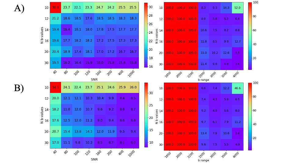
Figure 1. MAPE heat maps for A) hindered volume fraction and B) hindered diffusion coefficient for all simulations. Left: MAPE dependency on number and range of b-values; Right: MAPE dependency on b-values number and SNR.
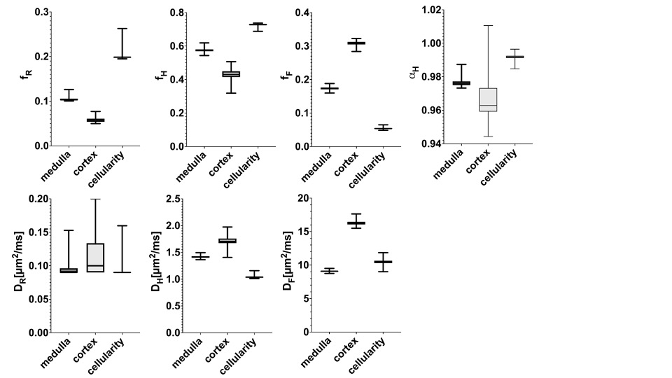
Figure 2. Statistical distribution of fitted parameters for three physiological conditions.
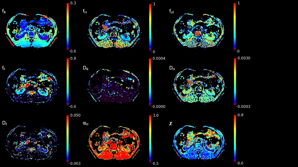
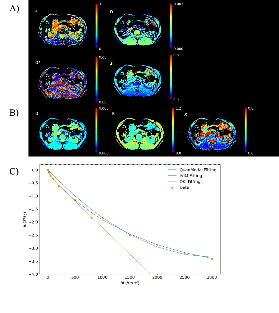
Figure 4. Example of the A) IVIM model parameters and B) DKI model parameters of kidney in a health adult. The last images are the rmse of fit; C) Comparison of fitting result in a single voxel for three models.
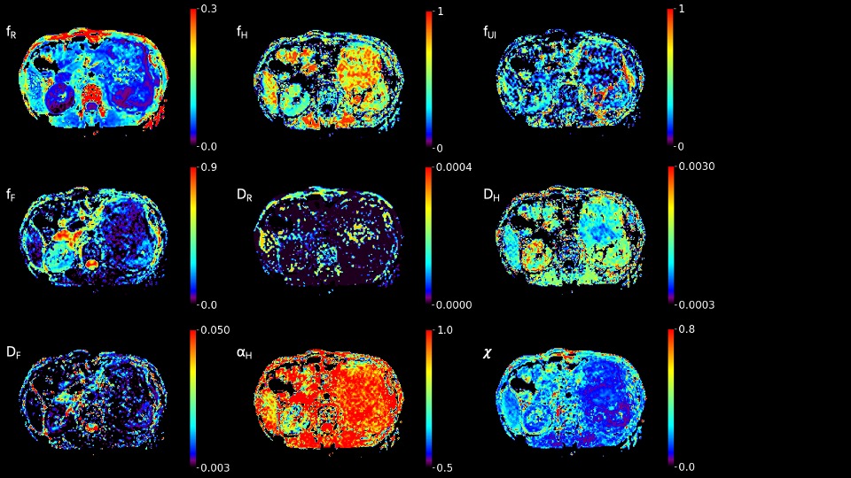
Figure 5. Example of the MAD model parameters of a patient with left kidney cancer where a mono-exponential ADC would not precisely represent the underlying micro-environment of lesion.