4434
Reliable Low-Field B0-Maps by Deep Learning with Physical Constraints
David Schote1, Lukas Winter1, Christoph Kolbitsch1, and Andreas Kofler1
1Physikalisch-Technische Bundesanstalt (PTB), Braunschweig and Berlin, Germany
1Physikalisch-Technische Bundesanstalt (PTB), Braunschweig and Berlin, Germany
Synopsis
Keywords: System Imperfections: Measurement & Correction, Low-Field MRI, B0-field map
Heavy B0-field inhomogeneities in low-field MRI can lead to geometric distortions in the reconstruction, if not compensated. We simulated low-field data to evaluate different approaches for estimating the field map from phase difference maps. By using spherical harmonic basis functions as physical constraints in our neural network approach we could improve the estimation of B0-field maps compared to other network architectures and methods not involving neural networks.Introduction
Low-field MRI devices can be affordably manufactured and are mobile, which increases the accessibility to MR imaging. The open-source low-field system OSI2 ONE 1-3 is built from permanent magnets in Halbach configuration. These systems usually suffer from relatively high B0-field inhomogeneities. In addition, permanent magnet properties depend on temperature which requires dynamic readjustments. If not compensated, the B0-field inhomogeneities can lead to geometric distortions in the acquired images. Temperature-independent effects can be canceled by time-consuming and system specific shimming 4. We propose methods for system-independent corrections by using neural networks (NN) to overcome these challenges.Methods
Spherical HarmonicsA phase difference map can be calculated from two acquisitions with different echo times and provides a first estimate of the magnetic field distribution. This B0-field map can be improved by a fit of spherical harmonic (SH) functions to ensure spatial smoothness. Due to the low SNR in low-field MRI, the problem of finding the SH coefficients and the B0-map from measurements is ill-posed. The problem can be solved by singular value decomposition (SVD), but due to the low SNR, this solution is not always optimal. Alternatively, the field map can be estimated by a neural network directly 5. Our approach overcomes the problem by estimating the coefficients from the measured phase difference maps using a NN. Hereby, the NN is constrained by a physical model. Using the estimated coefficients, we can calculate a high-quality B0-field map. The network follows a U-Net architecture with an encoder path and a fully connected layer providing the SH coefficients. We compared our approach to a network that directly estimates the B0-maps rather than the SH parameters. To exclude a possible performance increase of an NN-based method over another 6, we compared the two NN approaches at similar network capacity.
Finding the B0-field Map
It has been shown that SH coefficients can sufficiently describe the field distribution of Halbach systems up to the order of four 4. Based on the sphere radius $$$r$$$, the polar angle $$$\varphi$$$, and the azimuthal angle $$$\theta$$$, the B0-field map can be described by a weighted sum of real SH functions $$$Y_l^m$$$ and coefficients $$$c_l^m$$$. Since only projections for $$$\varphi=\frac{\pi}{2}$$$ are considered, the equation can be simplified.
$$\Delta B_0 (r, \theta, \varphi) = \sum_{l=0}^{L}\sum_{m=-l}^{m=l} (\frac{r}{r_0})^l c_l^m Y_l^m (\theta, \varphi)$$
Data
Based on a characterization of the low-field Halbach system7 we retrospectively simulated pairs of distorted low-field samples and ground truth images. Simulations are based on the FastMRI8 dataset and were performed in a similar fashion as described in Schote et al.9. The training dataset is supposed to cover a wide bandwidth of B0-fields with respect to the field strength and inhomogeneity distribution to ensure the applicability on different systems. To obtain random field maps in the range of a predefined scale, we apply exponential weighting, dependent on the coefficient order. Since also the SNR differs between systems, we modified the ground truth data by varying degrees of Gaussian noise. The overall process, including data simulation, field map estimation, and image reconstruction, which is carried out with the estimated field map, is visualized in figure 1.
Results
Figure 2 depicts the field map results by SVD, U-Net10, 11 and SH-Net compared to the ground truth. Calculating the coefficients by SVD results in a smooth field distribution but leads to errors in the regions with low signal intensities (e.g. outside air). Within a circular region of interest (RoI), structural errors become visible in the U-Net approach. Combining the strength of both approaches, the SH-Net delivers a smooth B0-field distribution with the best performance. Figure 3a shows the mean absolute error (MAE) within the RoI over a test dataset consisting of 180 samples. The SVD is compared to the U-Net architecture and our proposed architecture in terms of MAE. The results are evaluated at four different SNR levels. Both NN approaches lead to lower error boundaries and mean values than the SVD method. The MAE is the lowest and most stable with our SH-Net architecture for all the different noise levels. In Figure 3b we increased the capacity of the U-Net architecture. Thereby, an improvement of this architecture over our approach is gained only at low noise levels. Figure 4 compares the B0-field informed reconstruction by time segmentation for all field map estimations. As can be seen, by the error maps in the last row, errors from the field map estimates are propagated to the reconstructed images. This includes structural errors from the U-Net architecture. In contrast, our NN yields smooth field maps due to the explicit use of the generative model.Discussion and Conclusion
We could show the advanced performance of our proposed NN utilizing SH-model for B0 estimation in low-field MRI. Especially in the regime of low SNR, the NNs were able to achieve better results. By introducing physical constraints imposed by SH basis functions, we could achieve superior performance compared to only using a NN. Accurate results can be obtained for all the different considered noise levels. Structural errors from the U-Net approach which could propagate to the reconstructed image are inhibited by explicitly involving SH basis functions as physical constraints in our methodology.Acknowledgements
This work is part of the Metrology for Artificial Intelligence for Medicine (M4AIM) project that is funded by the Federal Ministery for Economic Affairs and Energy (BMWi) in the frame of the QI-Digital initiative.References
- T. O’Reilly, W. M. Teeuwisse, D. Gans, K. Koolstra, und A. G. Webb, „In vivo 3D brain and extremity MRI at 50 mT using a permanent magnet Halbach array“, Magn. Reson. Med., Bd. 85, Nr. 1, S. 495–505, Jan. 2021, doi: 10.1002/mrm.28396.
- T. O’Reilly, W. M. Teeuwisse, und A. G. Webb, „Three-dimensional MRI in a homogenous 27 cm diameter bore Halbach array magnet“, Journal of Magnetic Resonance, Bd. 307, S. 106578, Okt. 2019, doi: 10.1016/j.jmr.2019.106578.
- L. Winter, „Halbach array magnet for in vivo imaging“, Open-source imaging. https://www.opensourceimaging.org/project/halbach-array-magnet-for-in-vivo-imaging/ (zugegriffen 13. Oktober 2022).
- K. Wenzel, H. Alhamwey, T. O’Reilly, L. T. Riemann, B. Silemek, und L. Winter, „B0-Shimming Methodology for Affordable and Compact Low-Field Magnetic Resonance Imaging Magnets“, Front. Phys., Bd. 9, S. 704566, Juli 2021, doi: 10.3389/fphy.2021.704566.
- M. W. Haskell, A. A. Cao, D. C. Noll, und J. A. Fessler, „Deep learning field map estimation with model-based image reconstruction for off resonance correction of brain images using a spiral acquisition“, 2020.
- A. Kofler, T. Schaeffter, und C. Kolbitsch, „The More the Merrier? - On the Number of Trainable Parameters in Iterative Neural Networksfor Image Reconstruction“, in Proc. Intl. Soc. Mag. Reson. Med., London, 2022, Bd. 31, S. 0051.
- K. Koolstra, T. O’Reilly, P. Börnert, und A. Webb, „Image distortion correction for MRI in low field permanent magnet systems with strong B0 inhomogeneity and gradient field nonlinearities“, Magn Reson Mater Phy, Jan. 2021, doi: 10.1007/s10334-021-00907-2.
- J. Zbontar u. a., „fastMRI: An Open Dataset and Benchmarks for Accelerated MRI“, arXiv:1811.08839 [physics, stat], Dez. 2019, Zugegriffen: 17. November 2021. [Online]. Verfügbar unter: http://arxiv.org/abs/1811.08839
- D. Schote u. a., „Physics-Informed Deep Learning for Image Distortion Correction from B0-inhomogeneities in Low-Field MRI“, in Proc. Intl. Soc. Mag. Reson. Med., London, Bd. 31, S. 1816.
- M. P. Heinrich, M. Stille, und T. M. Buzug, „Residual U-Net Convolutional Neural Network Architecture for Low-Dose CT Denoising“, Current Directions in Biomedical Engineering, Bd. 4, Nr. 1, S. 297–300, Sep. 2018, doi: 10.1515/cdbme-2018-0072.
- O. Ronneberger, P. Fischer, und T. Brox, „U-Net: Convolutional Networks for Biomedical Image Segmentation“. arXiv, 18. Mai 2015. Zugegriffen: 18. Oktober 2022. [Online]. Verfügbar unter: http://arxiv.org/abs/1505.04597
Figures
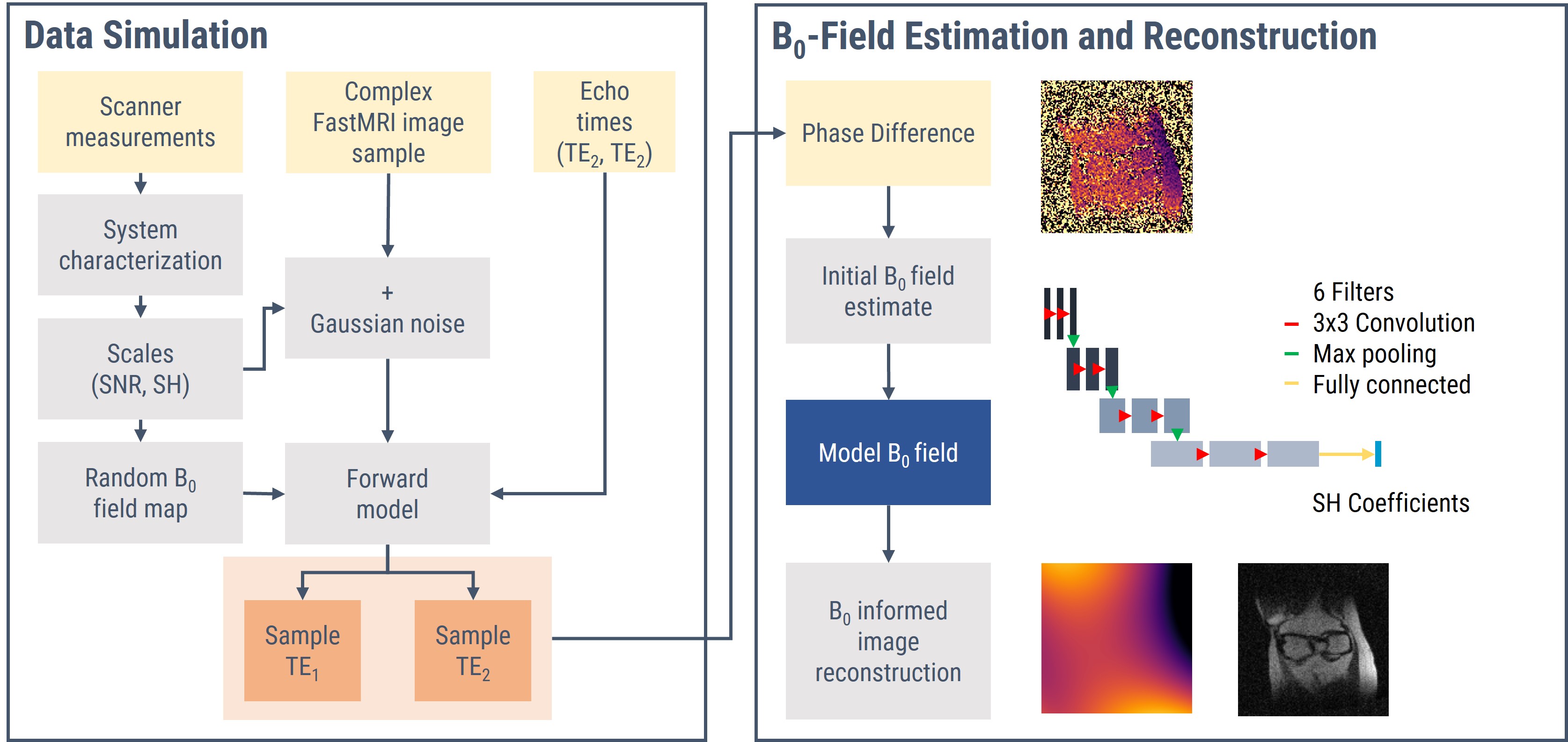
From randomized field maps, generated according to the
system characterization, and complex image samples, impaired by additional
Gaussian noise, two low-field samples are calculated by the forward model. From
phase difference, the field map is estimated and can be used for B0-informed
image reconstruction.
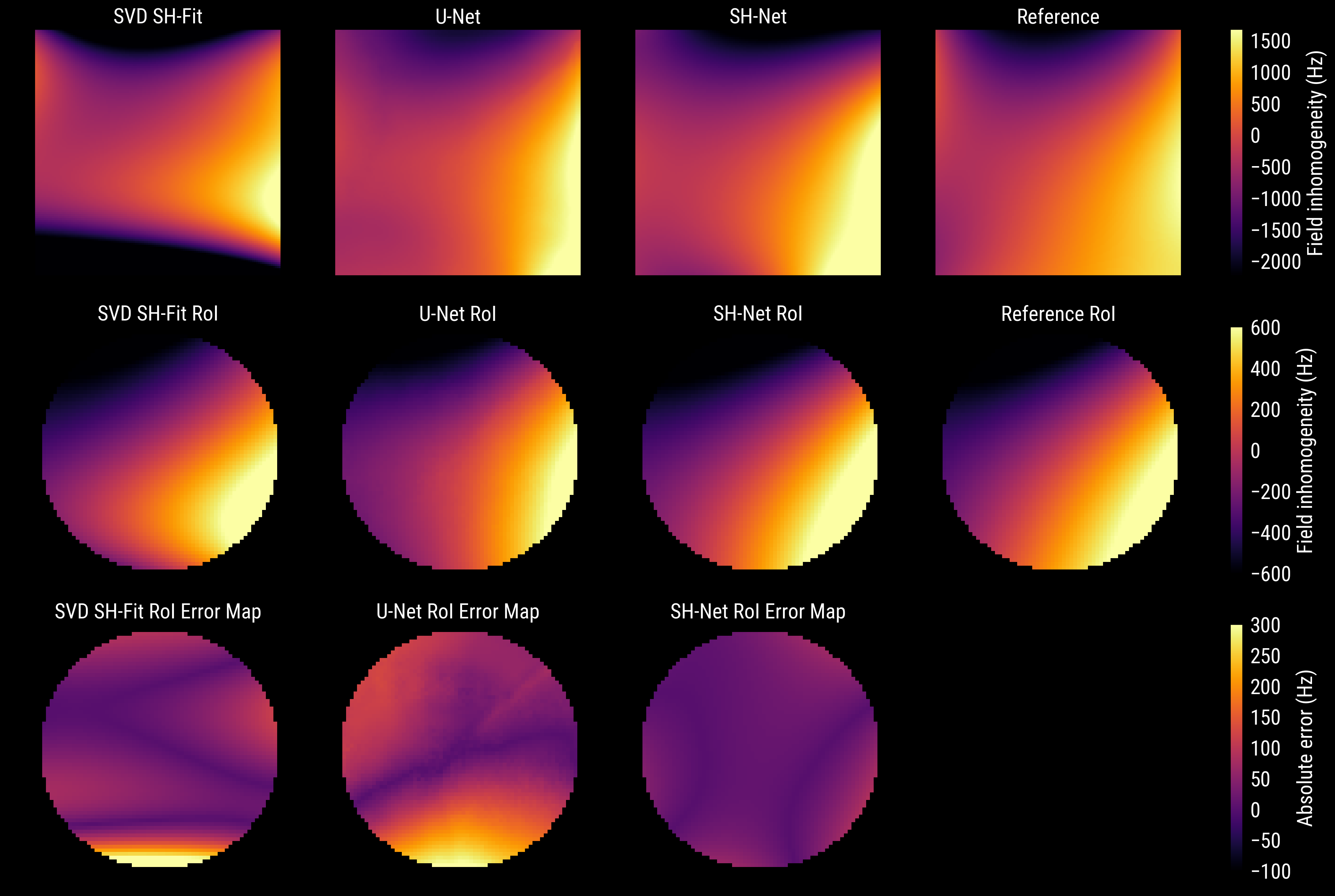
Field map estimation of a sample from the test dataset by SVD, U-Net, and SH-Net compared
to the reference. The first row shows the overall estimation of B0-field
inhomogeneity in Hz, the second row a circular RoI of it, and
the third row the absolute error to the reference inside the RoI. The RoI has a radius of 16 data points and the B0-field map dimension is 128 times 128.
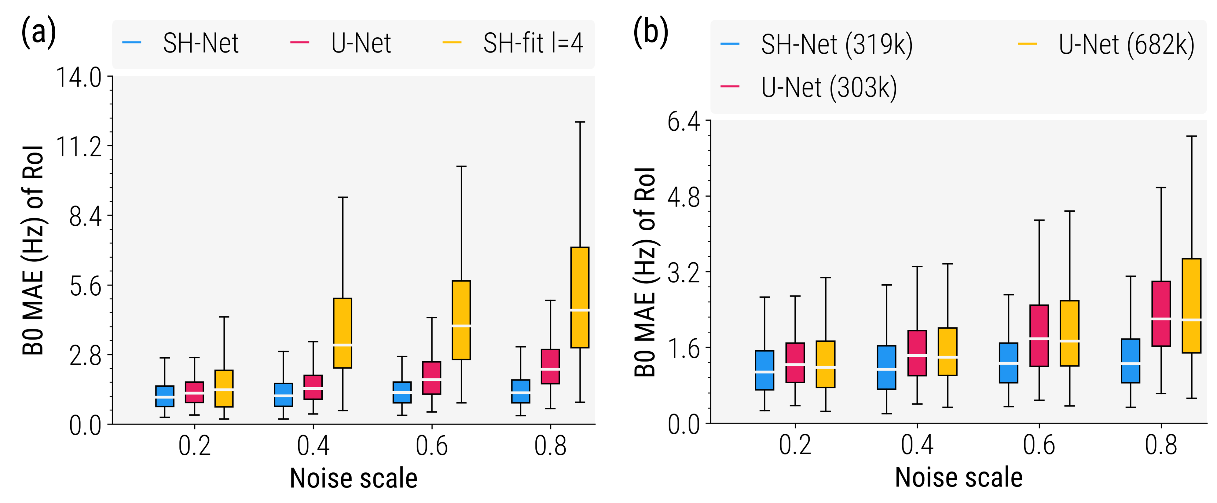
Mean absolute error (MAE) of the B0-field map inside a
circular RoI with a radius of 16 data points. Figure (a) reveals
improved performance and stability in comparison to a U-Net with similar parameters and the estimation by SVD that
becomes more significant with the increasing noise level. Figure (b) indicates a
performance limit of the U-Net as there is only an improvement for the lowest
noise level and no difference at higher noise levels.
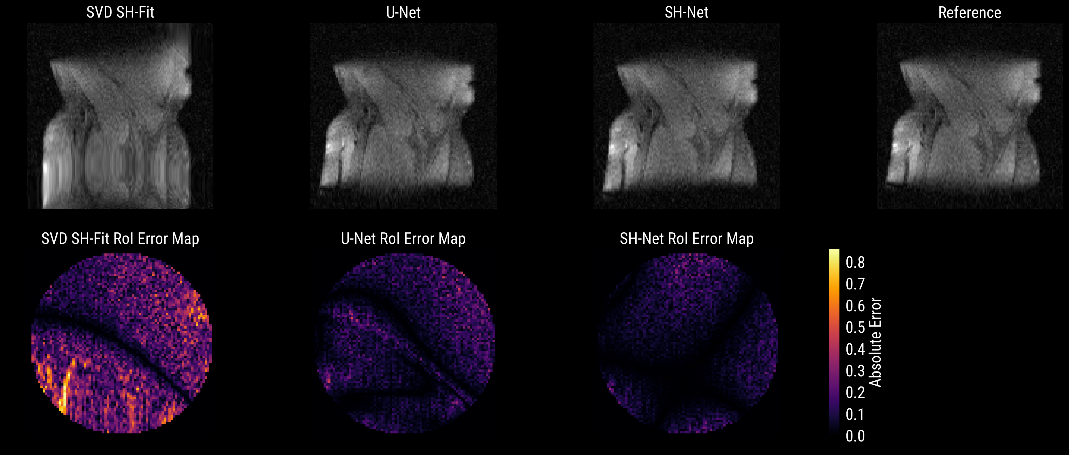
Comparison of B0-field informed image
reconstruction based on time segmentation. A comparison of the magnitude images
to ground truth is shown in the first row. The error maps within the corresponding circular RoI are shown in the second row and reveal the error propagation
from field map estimation to image. The RoI has a radius of 16 data points and the B0-field map dimension is 128 times 128.
DOI: https://doi.org/10.58530/2023/4434