Synopsis

Keywords: Diffusion/other diffusion imaging techniques, Simulations, Time-dependence diffusion

We segment all myelinated and unmyelinated axons from electron microscopy (EM) images of brain white matter (WM) of a mouse and a rat and quantify their cross-sectional morphology. We provide the exact relation between the long-time limit of the along-axon diffusion coefficients and the geometry of segmented intra-axonal spaces (IAS). By performing Monte Carlo (MC) simulations of diffusion in the IASs at varying diffusion times, we establish the time-dependence of diffusion along segmented myelinated and unmyelinated axons and validate the relation between axonal geometry and the long-time behavior of the longitudinal diffusion coefficient.

INTRODUCTION

Diffusion MRI (dMRI) is sensitive to the micro-scale geometry of brain tissue as the diffusion length is commensurate with the cell size. However, ensemble averaging of the diffusion propagator irreversibly coarse-grains heterogeneities of the tissue structural properties¹. Biophysical modeling¹ enables quantifying such properties much below the nominal resolution of MRI. While early works^2,3 of modeling dMRI in WM described diffusion along axons as Gaussian as a 1-dimensional (1d) impermeable cylinder, recently, the structural disorder of the IAS in myelinated axons was uncovered⁴ and tied⁵ to the $$$1/\sqrt{t}$$$ dependence^6,7 of the along-axon diffusion coefficient $$$D(t)$$$. However, the challenge has remained to investigate the role of unmyelinated axons in the observed WM dMRI signal, as their segmentation is far more difficult due to their thin walls. Furthermore, although the relation between the IAS geometry and the Gaussian $$$D_\infty=D\left(t\right)|_{t\rightarrow\infty}$$$ has been approximated in ref⁵, their exact relation has remained to be solved. For the first time, we segment all myelinated and unmyelinated axons in the corpus callosum of a mouse⁴ and a rat⁸ acquired by EM and quantify their cross-sectional morphology, such as beading. We drive the exact relation between the IAS geometry and $$$D\left(t\right)|_{t\rightarrow\infty}$$$ based on Fick-Jacob’s equation, and by performing MC simulations of diffusion⁹ in the IASs at $$$t\le100$$$ ms, we validate our findings.

METHODS

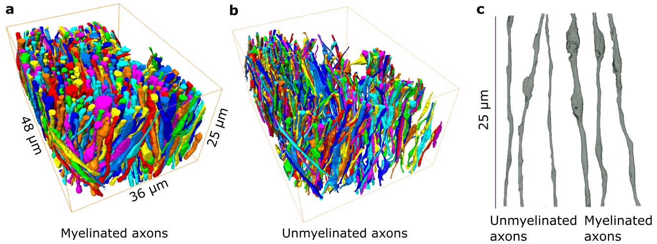
EM: We acquired two samples from the corpus callosum: 48μm×36μm×25μm sample of an adult mouse imaged at 6nm×6nm×100nm⁴ and 15μm×15 μm×25μm sample from an adult rat at imaged 15nm×15nm×50nm.
EM segmentation: We apply a deep learning-based approach for the semantic segmentation of IASs and employ a percentile-based agglomeration technique for their instance segmentation^8,10.
MC simulations: 200,000 random walkers per axon for $$$t\le100$$$ ms simulate diffusion in a continuous 3d space⁹.
Fick-Jacob’s equation: We consider narrow axons with varying cross-sections $$$A(x)$$$ along the length $$$x$$$, for which diffusion quickly homogenizes the 3d particle density $$$n(x,x_\perp)\approx n(x)$$$ in each cross-section, making it independent of the transverse coordinate $$$x_\perp$$$, such that the relevant 1d density $$$\psi(x)=n(x)A(x)$$$. The current $$$J(x)=-D_0A(x)\partial_x\left(\frac{\psi(x)}{A(x)}\right)$$$ defines the FJ's equation, $$$D_0$$$ is free diffusivity, for $$$\psi(x)$$$: $$\partial_t\psi(t,x)=D_0\partial_x\left[A(x) \partial_x \left(\frac{\psi(x)}{A(x)}\right)\right].\qquad(1)$$
Tortuosity limit: For $$$t\to\infty$$$, the transient processes die out, $$$\partial_t\psi\equiv0$$$, and the current in each cross-section $$$J(x)=\mathrm{const}$$$. Now, defining the overall density difference along an axon as $$$\Delta n$$$, we write it as the sum of local densities $$$\Delta n=\Delta n_1+\Delta n_2+\dots$$$. Let us split an axon into small segments of lengths $$$l_i$$$ and cross-sections $$$A_i$$$. For $$$t\rightarrow\infty$$$, $$$J\left(x\right)=const$$$, in each cross-section, therefore $$J\equiv D_0A_1\frac{\Delta n_1}{l_1}=D_0A_2\frac{\Delta n_2}{l_2}=\ldots\Rightarrow\Delta n_i=\frac{J}{D_0}\frac{\Delta l_i}{A_i}\Rightarrow\sum{\Delta n_i}=\frac{J}{D_0}\sum\left(\frac{\Delta l_i}{A_i}\right).$$
Also, for $$$t\rightarrow\infty$$$, we have $$$\Delta n=\frac{J}{D_\infty}\frac{\sum l_i}{\bar{A}}$$$, which defines $$$D_\infty$$$. Thus, we get: $$\frac{D_0}{D_\infty}=\frac{\bar{A}}{\sum l_i}\sum\frac{l_i}{A_i}\Rightarrow\frac{D_0}{D_\infty}=\left\langle\frac{\bar{A}}{A\left(x\right)}\right\rangle.$$
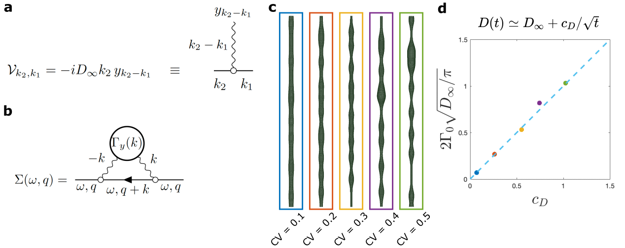
The time-dependent approach of $$$D(t)$$$ to $$$D_\infty$$$: Working at long $$$t$$$ effectively around $$$D(t)\simeq D_\infty$$$, the coarse-grained fluctuations of $$$A(x)$$$ become small, such that we can substitute $$$D_0\to D_\infty$$$ and present Eq.1 as $$\partial_t\psi(t,x)=D_\infty\partial^2_x\psi(x)-D_\infty\partial_x\left[y(x)\psi(t,x)\right]\,,\quad y(x) = \partial_x\ln(1+\alpha(x))\simeq\partial_x\alpha(x)\,,$$ where $$$\alpha(x)=[A(x)-\overline{A}]/\overline{A}$$$ is a relative area fluctuation, and $$$\overline{A}=\int_0^L\! dx\,A(x)/L$$$ is the mean cross-section area. The last term defines the perturbation $$\mathcal{V}\psi\equiv-D_\infty\partial_x\left[y(x)\psi(t,x)\right]\,.$$ In the Fourier domain, this corresponds to the scattering term $$\mathcal{V}_{k_2,k_1}=-iD_\infty k_2\, y_{k_2-k_1},$$ where the wavy line in Fig.5a represents an elementary scattering event with an incoming momentum $$$k_2-k_1$$$ transferred to the particle with momentum $$$k_1$$$, such that it proceeds with momentum $$$k_2$$$. The corresponding self-energy part (shown in Fig.5b) $$\Sigma(\omega,q)=-D_\infty^2\int\!\frac{dk}{2\pi}\,\frac{q(k+q)\,\Gamma_y(k)}{-i\omega+D_\infty(k+q)^2},$$ where $$\Gamma_y(k)=\frac{y(k)y(k)}L\,\simeq k^2 \frac{\alpha(-k)\alpha(k)}L\,\equiv k^2\,\Gamma_\alpha(k)$$ is the power spectral density of $$$y(x)$$$. Expanding $$$\Sigma(\omega,q)$$$ up to $$$\mathcal{O}(q^2)$$$ provides the dispersive contribution to the overall diffusivity $$$\mathcal{D}(\omega)$$$¹, which results in $$D(t)\simeq D_\infty+\frac{c_D}{\sqrt{t}}\qquad(2)$$ for the short-range disorder in $$$\alpha(x)$$$, similar to Ref⁶, where $$c_D=2\Gamma_0\,\sqrt{\frac{D_\infty}\pi}\,$$ and $$$\Gamma_0=\lim_{k\to0}\Gamma_\alpha(k)$$$ (with dimensions of length) is the plateau of the power spectrum of $$$\alpha(x)$$$ at low $$$k$$$.

RESULTS

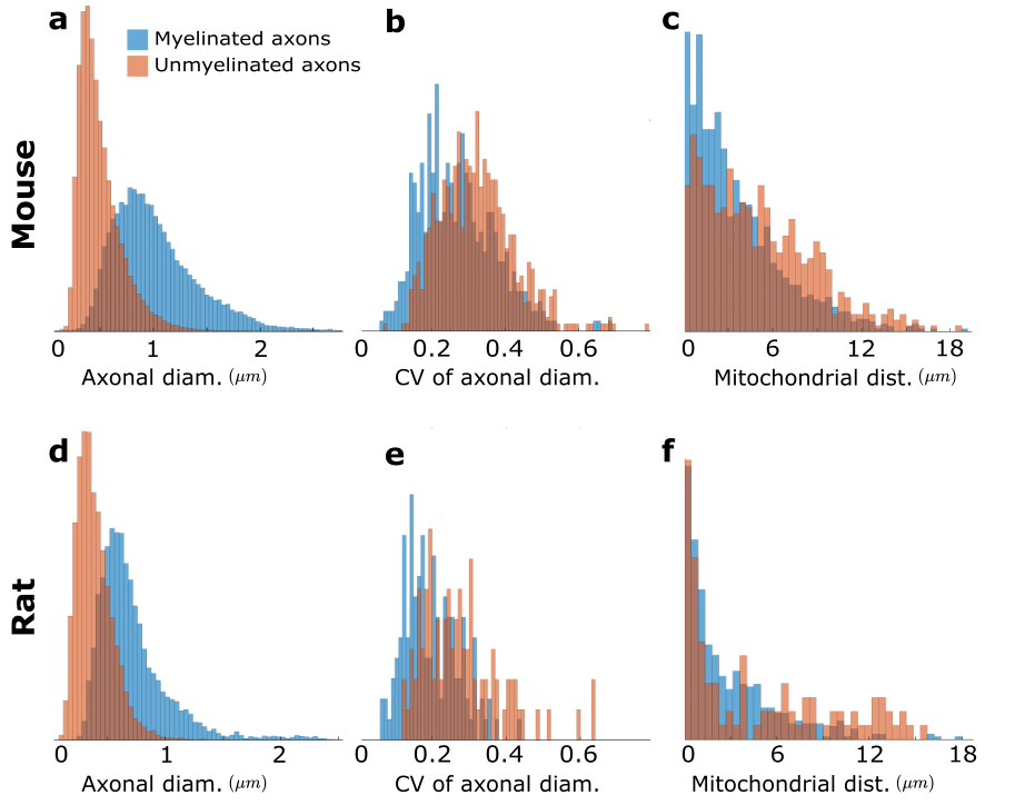
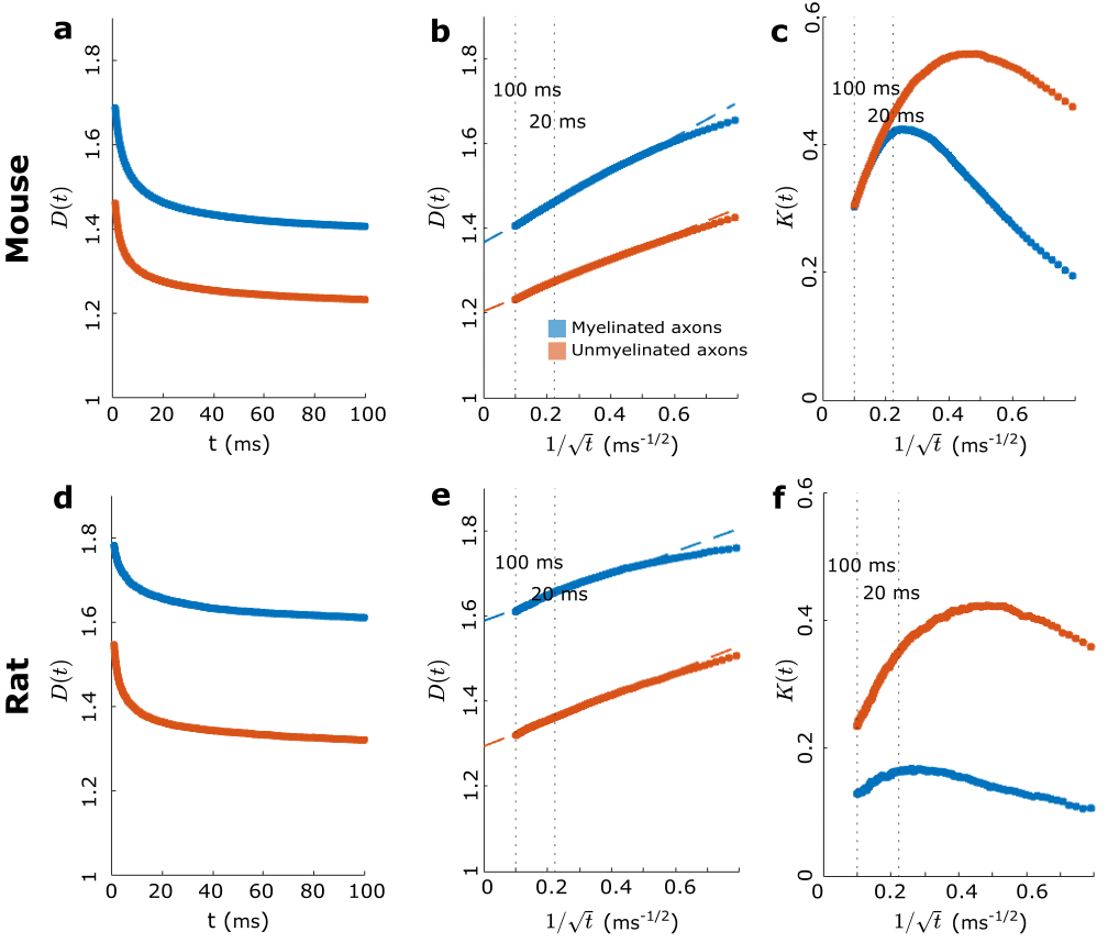
We used segmented axons longer than 20μm for morphometry and MC simulations (Fig.1). Fig.2 shows that the IASs' diameter (dataset: mean±std) is (mouse: 1.03±0.40μm; rat: 0.71±0.31μm) for myelinated and (mouse: 0.52±0.21μm; rat: 0.39±0.15μm) for unmyelinated axons. The coefficient of variation (CV) corresponding to beading is (mouse: 0.27±0.10; rat: 0.20±0.07) for myelinated and (mouse: 0.32±0.10; rat:0.28±0.11) for unmyelinated axons. The distance between mitochondria along myelinated axons is (mouse:4.57±3.99 μm; rat: 2.84±2.97μm), and for unmyelinated axons is (mouse: 6.47±4.74μm; rat: 4.78±4.72μm). Thus, unmyelinated axons are twice thinner, have stronger beading, and have a larger mitochondrial distance than myelinated axons.

MC simulations of $$$D(t)$$$ exhibit notable time-dependence along axons, scaling as $$$1/\sqrt{t}$$$ (Fig.3), and are consistent with the short-range disorder in $$$A(x)$$$. The smaller $$$D(t)$$$ and $$$D_\infty$$$ of unmyelinated axons implies stronger diffusion, in line with their stronger beadings.

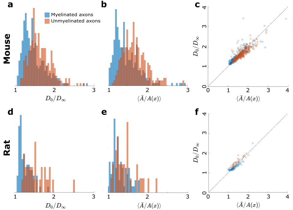
We extrapolate $$$D(t)$$$ as a function of $$$1/\sqrt{t}$$$ to determine $$$D_\infty$$$, hence the tortuosity limit $$$D_0/D_\infty$$$ (Fig.4a). Unmyelinated axons have a higher tortuosity, corresponding to their stronger beadings (Fig.4b). We validate the derivation of the exact tortuosity limit in relation to the IAS geometry in Fig.4c.

In Fig.5, we synthetically generate five long (500 μm) axons with the statistics of the real axons (Fig.2). We validate $$$c_D$$$ in Eq.2 by simulating $$$D(t)$$$ in these synthetic axons and comparing the results to the plateau of $$$\Gamma_0=\lim_{k\to0}\Gamma_\alpha(k)$$$, as shown in Fig.5d for different beading strengths.

CONCLUSION

Realistic axonal geometries enabled us to establish diffusion time-dependence and validate the relation between axonal geometry and long-time $$$D(t)$$$.

Acknowledgements

This work was supported by NIH R21 NS081230, R01 NS088040, NIH OD and NIDCR DP5OD031854, and was performed at the Center of Advanced Imaging Innovation and Research, an NIBIB Biomedical Technology Resource Center (NIH P41 EB017183).