4314
Twinkle, twinkle, T2*, still we wonder what you are1Department of Radiology, New York University School of Medicine, New York, NY, United States
Synopsis
Keywords: Microstructure, Relaxometry, T2* decay
In the absence of macroscopic magnetic field inhomogeneity, the decay of gradient-echo signals is generally observed to be approximately monoexponential, with time constant $$$T_2^*$$$. The monoexponential behavior is typically attributed to diffusion, which averages out the dephasing of spins due to microstructural sources of magnetic susceptibility. The rationale is that, over times long enough for spins to have explored the microstructure, the cumulants of the spins’ phase distribution should increase linearly with time. By means of a simple counterexample, we demonstrate that this assumption is incorrect, thereby calling into question the mechanism underlying the monoexponential decay of gradient-echo signals.Introduction
In the absence of macroscopic magnetic field inhomogeneity, the gradient-echo signal is generally well approximated by a monoexponential decay, with time constant $$$T_2^*$$$. One contribution to the decay stems from transverse relaxation on a molecular scale due to dipole-dipole interactions$$$^1$$$. Another component arises from spin dephasing due to micron-scale magnetic field heterogeneity, which results from microstructural sources of magnetic susceptibility$$$^{2-8}$$$$$S\left(t\right)=S_0\,e^{-t/T_2}\left\langle\,\!e^{i\phi\left(t\right)}\right\rangle\;\;\;\;\;\;\;\;\left[1\right]$$
where
$$\phi\left(t\right)=\int_0^t\mathrm{d}t^{\prime}\,\Omega\left(t^{\prime}\right)$$
and
$$\Omega\left(t\right)=\gamma\,\Delta B\left[\mathbf{r}\left(t\right)\right]$$
Without loss of generality, we may assume $$$\left\langle\Delta B\left(\mathbf{r}\right)\right\rangle=0$$$, which ensures that $$$\left\langle\phi\left(t\right)\right\rangle=0$$$.
In describing the effect of field heterogeneity on signal decay, it is useful to define a correlation time $$$\tau_c=L^2/D$$$, which represents the interval required for spins to diffuse a distance equal to the characteristic length scale $$$L$$$ of the microstructure, where $$$D$$$ is the diffusion coefficient. Over times $$$t\sim\tau_c$$$, the form of the signal decay is sensitive to short-range variations in magnetic field. However, as time increases, diffusion allows spins to explore the microstructure. This motional averaging is believed to underlie the observed monoexponential behavior of the signal at long times$$$^{8,9}$$$, i.e. $$$ t\gg\tau_c$$$.
The strength of the signal perturbations due to the microstructure may be quantified by the parameter $$$\alpha=\delta\Omega\,\tau_c$$$, where $$$\delta\Omega^2=\left\langle\Omega^2\left(\mathbf{r}\right)\right\rangle$$$ is the variance in Larmor frequency. Thus $$$\alpha$$$ represents the amount of dephasing that occurs over the correlation time.
In the weak field approximation, $$$\alpha\ll1$$$, the ensemble average in [1] may be replaced by a cumulant expansion$$$^{3-8}$$$
$$\left\langle\,\!e^{i\phi\left(t\right)}\right\rangle=\exp\left[\sum_{n=1}^{\infty}\frac{\left(i\right)^n}{n!}\kappa_n\left(t\right)\right]\;\;\;\;\;\;\;\;\left[2\right]$$
where the odd-order cumulants can be ignored if only the magnitude of the signal is of interest.
The second-order cumulant equals the variance
$$\kappa_2\left(t\right)=\left\langle\phi^2\left(t\right)\right\rangle$$
and the fourth-order cumulant is given by
$$\kappa_4\left(t\right)=\left\langle\phi^4\left(t\right)\right\rangle-3\left\langle\phi^2\left(t\right)\right\rangle^2$$
where terms containing the mean phase have been dropped, since $$$\left\langle\phi\left(t\right)\right\rangle=0$$$.
The conventional explanation for monoexponential signal decay is that, for $$$t/\tau_c\rightarrow\infty$$$, the total time can be divided into many intervals, each one equal to $$$\tau_c$$$ (or some multiple thereof). Since $$$\tau_c$$$ represents the time scale over which $$$\Omega\left(t+\tau_c\right)$$$ becomes statistically independent from $$$\Omega\left(t\right)$$$, the phases accrued by spins in each interval should be uncorrelated. Because cumulants of independent random variables add, all the cumulants should scale linearly with time for $$$t\gg\tau_c$$$. From [1] and [2], it follows that the signal must decay monoexponentially, at a rate $$$R_2^*=1/T_2^*$$$ that contains contributions from all even-order cumulants$$$^8$$$.
In this work, we demonstrate the fallacy of this argument by means of a simple counterexample, namely free diffusion through magnetic field perturbations consisting of spatially-correlated Gaussian-distributed noise (Figure 1). Specifically, we show that the argument fails for $$$\kappa_{n>2}(t)$$$.
Theory
The phase variance can be expressed in terms of the temporal frequency covariance$$$^{5,8}$$$ as$$\begin{split}\left\langle\phi^2\left(t\right)\right\rangle&=\int_0^t\mathrm{d}t_1\int_0^t\mathrm{d}t_0\,\left\langle\Omega\left(t_0\right)\Omega\left(t_1\right)\right\rangle\\&=2!\int_0^t\mathrm{d}t_1\int_0^{t_1}\mathrm{d}t_0\,\left\langle\Omega\left(t_0\right)\Omega\left(t_1\right)\right\rangle\end{split}$$
The temporal covariance can in turn be written in terms of the spatial covariance
$$\left\langle\Omega\left(t_0\right)\Omega\left(t_1\right)\right\rangle=\int\mathrm{d}^3\mathbf{r}_1\left\langle\Omega\left(\mathbf{r}_0\right)\Omega\left(\mathbf{r}_1\right)\right\rangle\,\!D\left(\mathbf{r}_1-\mathbf{r}_0,t_1-t_0\right)\;\;\;\;\;\;\;\;\left[3\right]$$
where
$$D\left(\mathbf{r},\tau\right)=\frac{e^{-\left|\mathbf{r}\right|^2/4D\tau}}{\left(4\pi\,\!D\tau\right)^{3/2}}$$
is the diffusion propagator. For field perturbations consisting of spatially-correlated Gaussian-distributed noise,
$$\left\langle\Omega\left(\mathbf{r}_0\right)\Omega\left(\mathbf{r}_0+\mathbf{r}\right)\right\rangle=\delta\Omega^2\,e^{-\left|\mathbf{r}\right|^2/4L^2}$$
Substitution into [3] gives
$$\left\langle\Omega\left(t_0\right)\Omega\left(t_0+\tau\right)\right\rangle=\frac{\delta\Omega^2}{\left(1+\tau/\tau_c\right)^{3/2}}\;\;\;\;\;\;\;\;\left[4\right]$$
and integration over time yields
$$\left\langle\phi^2\left(t\right)\right\rangle=4\alpha^2\left(\frac{t}{\tau_c}-2\sqrt{1+\frac{t}{\tau_c}}+2\right)$$
Note that $$$\left\langle\phi^2\left(t\right)\right\rangle\propto\alpha^2$$$. More generally, $$$\kappa_n\left(t\right)\propto\alpha^n$$$.
Since
$$\lim_{t/\tau_c\rightarrow\infty}\left(\frac{\mathrm{d}}{\mathrm{d}t}\left\langle\phi^2\left(t\right)\right\rangle\right)=\frac{4\alpha^2}{\tau_c}$$
the variance increases linearly with time for $$$t\gg\tau_c$$$.
The fourth-order cumulant can be calculated in an analogous fashion. Consider first the fourth moment
$$\begin{split}\left\langle\phi^4\left(t\right)\right\rangle&=\int_0^t\mathrm{d}t_3\int_0^t\mathrm{d}t_2\int_0^t\mathrm{d}t_1\int_0^t\mathrm{d}t_0\,\left\langle\Omega\left(t_0\right)\Omega\left(t_1\right)\Omega\left(t_2\right)\Omega\left(t_3\right)\right\rangle\\&=4!\int_0^t\mathrm{d}t_3\int_0^{t_3}\mathrm{d}t_2\int_0^{t_2}\mathrm{d}t_1\int_0^{t_1}\mathrm{d}t_0\,\left\langle\Omega\left(t_0\right) \Omega\left(t_1\right) \Omega\left(t_2\right) \Omega\left(t_3\right)\right\rangle\end{split}$$
The integrand can be expressed in terms of a joint probability distribution at different spatial locations,
$$\begin{split}\left\langle\Omega\left(t_0\right)\Omega\left(t_1\right)\Omega\left(t_2\right)\Omega\left(t_3\right)\right\rangle=\int\mathrm{d}^3\mathbf{r}_3\int\mathrm{d}^3\mathbf{r}_2\int\mathrm{d}^3\mathbf{r}_1&\left\langle\Omega\left(\mathbf{r}_0\right)\Omega\left(\mathbf{r}_1\right)\Omega\left(\mathbf{r}_2\right)\Omega\left(\mathbf{r}_3\right)\right\rangle\times\\&D\left(\mathbf{r}_1-\mathbf{r}_0,t_1-t_0\right)D\left(\mathbf{r}_2-\mathbf{r}_1,t_2-t_1\right)D\left(\mathbf{r}_3-\mathbf{r}_2,t_3-t_2\right)\end{split}$$
Since the field perturbations consist of spatially-correlated Gaussian-distributed noise, this joint probability is a multivariate Gaussian, which can be decomposed into three terms
$$\begin{split}\left\langle\Omega\left(\mathbf{r}_0\right)\Omega\left(\mathbf{r}_1\right)\Omega\left(\mathbf{r}_2\right)\Omega\left(\mathbf{r}_3\right)\right\rangle&=\left\langle\Omega\left(\mathbf{r}_0\right)\Omega\left(\mathbf{r}_1\right)\right\rangle\left\langle\Omega\left(\mathbf{r}_2\right)\Omega\left(\mathbf{r}_3\right)\right\rangle\\&+\left\langle\Omega\left(\mathbf{r}_0\right)\Omega\left(\mathbf{r}_2\right)\right\rangle\left\langle\Omega\left(\mathbf{r}_1\right)\Omega\left(\mathbf{r}_3\right)\right\rangle\\&+\left\langle\Omega\left(\mathbf{r}_0\right)\Omega\left(\mathbf{r}_3\right)\right\rangle\left\langle\Omega\left(\mathbf{r}_1\right)\Omega\left(\mathbf{r}_2\right)\right\rangle\end{split}$$
as represented in Figure 2. Thus
$$\left\langle\Omega\left(t_0\right)\Omega\left(t_1\right)\Omega\left(t_2\right)\Omega\left(t_3\right)\right\rangle=\left\langle\Omega\left(t_0\right)\Omega\left(t_1\right)\Omega\left(t_2\right)\Omega\left(t_3\right)\right\rangle_{\left(0,1\right)\left(2,3\right)}+\left\langle\Omega\left(t_0\right)\Omega\left(t_1\right)\Omega\left(t_2\right)\Omega\left(t_3\right)\right\rangle_{\left(0,2\right)\left(1,3\right)}+\left\langle\Omega\left(t_0\right)\Omega\left(t_1\right)\Omega\left(t_2\right)\Omega\left(t_3\right)\right\rangle_{\left(0,3\right)\left(1,2\right)}$$
where
$$\begin{split}\left\langle\Omega\left(t_0\right)\Omega\left(t_1\right)\Omega\left(t_2\right)\Omega\left(t_3\right)\right\rangle_{\left(i,j\right)\left(k,l\right)}=\int\mathrm{d}^3\mathbf{r}_3\int\mathrm{d}^3\mathbf{r}_2\int\mathrm{d}^3\mathbf{r}_1&\left\langle\Omega\left(\mathbf{r}_i\right)\Omega\left(\mathbf{r}_j\right)\right\rangle\left\langle\Omega\left(\mathbf{r}_k\right)\Omega\left(\mathbf{r}_l\right)\right\rangle\times\\&D\left(\mathbf{r}_1-\mathbf{r}_0,t_1-t_0\right)D\left(\mathbf{r}_2-\mathbf{r}_1,t_2-t_1\right)D\left(\mathbf{r}_3-\mathbf{r}_2,t_3-t_2\right)\end{split}$$
These equal
$$\begin{split}\left\langle\Omega\left(t_0\right)\Omega\left(t_1\right)\Omega\left(t_2\right)\Omega\left(t_3\right)\right\rangle_{\left(0,1\right)\left(2,3\right)}&=\frac{\delta\Omega^4}{\left[\left(1+\frac{\tau_1}{\tau_c}\right)\left(1+\frac{\tau_3}{\tau_c}\right)\right]^{3/2}}\\\left\langle\Omega\left(t_0\right)\Omega\left(t_1\right)\Omega\left(t_2\right)\Omega\left(t_3\right)\right\rangle_{\left(0,2\right)\left(1,3\right)}&=\frac{\delta\Omega^4}{\left[\left(1+\frac{\tau_1+\tau_2}{\tau_c}\right)\left(1+\frac{\tau_2+\tau_3}{\tau_c}\right)-\left(\frac{\tau_2}{\tau_c}\right)^2\right]^{3/2}}\\\left\langle\Omega\left(t_0\right)\Omega\left(t_1\right)\Omega\left(t_2\right)\Omega\left(t_3\right)\right\rangle_{\left(0,3\right)\left(1,2\right)}&=\frac{\delta\Omega^4}{\left[\left(1+\frac{\tau_1+\tau_2+\tau_3}{\tau_c}\right)\left(1+\frac{\tau_2}{\tau_c}\right)-\left(\frac{\tau_2}{\tau_c}\right)^2\right]^{3/2}}\end{split}$$
where
$$\begin{split}\tau_1&=t_1-t_0\\\tau_2&=t_2-t_1\\\tau_3&=t_3-t_2\end{split}$$
The variance squared can similarly be expressed as a four-dimensional integral with three analogous terms
$$\begin{split}\left\langle\phi^2\left(t\right)\right\rangle^2&=\int_0^t\mathrm{d}t_3\int_0^t\mathrm{d}t_2\int_0^t\mathrm{d}t_1\int_0^t\mathrm{d}t_0\,\left\langle\Omega\left(t_0\right)\Omega\left(t_1\right)\right\rangle\left\langle\Omega\left(t_2\right)\Omega\left(t_3\right)\right\rangle\\&=\frac{4!}{3}\int_0^t\mathrm{d}t_3\int_0^{t_3}\mathrm{d}t_2\int_0^{t_2}\mathrm{d}t_1\int_0^{t_1}\mathrm{d}t_0\,\left[\left\langle\Omega\left(t_0\right)\Omega\left(t_1\right)\right\rangle\left\langle\Omega\left(t_2\right)\Omega\left(t_3\right)\right\rangle+\left\langle\Omega\left(t_0\right)\Omega\left(t_2\right)\right\rangle\left\langle\Omega\left(t_1\right)\Omega\left(t_3\right)\right\rangle+\left\langle\Omega\left(t_0\right)\Omega\left(t_3\right)\right\rangle\left\langle\Omega\left(t_1\right)\Omega\left(t_2\right)\right\rangle\right]\end{split}$$
From equation [4],
$$\begin{split}\left\langle\Omega\left(t_0\right)\Omega\left(t_1\right)\right\rangle\left\langle\Omega\left(t_2\right)\Omega\left(t_3\right)\right\rangle&=\frac{\delta\Omega^4}{\left[\left(1+\frac{\tau_1}{\tau_c}\right)\left(1+\frac{\tau_3}{\tau_c}\right)\right]^{3/2}}\\\left\langle\Omega\left(t_0\right)\Omega\left(t_2\right)\right\rangle\left\langle\Omega\left(t_1\right)\Omega\left(t_3\right)\right\rangle&=\frac{\delta\Omega^4}{\left[\left(1+\frac{\tau_1+\tau_2}{\tau_c}\right)\left(1+\frac{\tau_2+\tau_3}{\tau_c}\right)\right]^{3/2}}\\\left\langle\Omega\left(t_0\right)\Omega\left(t_3\right)\right\rangle\left\langle\Omega\left(t_1\right)\Omega\left(t_2\right)\right\rangle&=\frac{\delta\Omega^4}{\left[\left(1+\frac{\tau_1+\tau_2+\tau_3}{\tau_c}\right) \left(1+\frac{\tau_2}{\tau_c}\right)\right]^{3/2}}\end{split}$$
Note that
$$\begin{split}\left\langle\Omega\left(t_0\right)\Omega\left(t_1\right)\Omega\left(t_2\right)\Omega\left(t_3\right)\right\rangle_{\left(0,1\right)\left(2,3\right)}&=\left\langle\Omega\left(t_0\right)\Omega\left(t_1\right)\right\rangle\left\langle\Omega\left(t_2\right)\Omega\left(t_3\right)\right\rangle\;\;\;\;\;\;\;\;\left[5a\right]\\\left\langle\Omega\left(t_0\right)\Omega\left(t_1\right)\Omega\left(t_2\right)\Omega\left(t_3\right)\right\rangle_{\left(0,2\right)\left(1,3\right)}&\neq\left\langle\Omega\left(t_0\right)\Omega\left(t_2\right)\right\rangle\left\langle\Omega\left(t_1\right)\Omega\left(t_3\right)\right\rangle\;\;\;\;\;\;\;\;\left[5b\right]\\\left\langle\Omega\left(t_0\right)\Omega\left(t_1\right)\Omega\left(t_2\right)\Omega\left(t_3\right)\right\rangle_{\left(0,3\right)\left(1,2\right)}&\neq\left\langle\Omega\left(t_0\right)\Omega\left(t_3\right)\right\rangle\left\langle\Omega\left(t_1\right)\Omega\left(t_2\right)\right\rangle\;\;\;\;\;\;\;\;\left[5c\right]\end{split}$$
Hence the contributions from the quantities in [5a] to the fourth-order cumulant $$$\kappa_4\left(t\right)=\left\langle\phi^4\left(t\right)\right\rangle-3\left\langle\phi^2\left(t\right)\right\rangle^2$$$ cancel. The quantities in [5b] and [5c] differ only by the term $$$\left(\tau_2/\tau_c\right)^2$$$ in the denominator, so their contributions to $$$\kappa_4\left(t\right)$$$ partially cancel.
Methods
The fourth-order cumulant $$$\kappa_4\left(t\right)$$$ and its time-derivative $$$\kappa_4^{\prime}\left(t\right)$$$ were computed numerically from the integral expressions above over the interval $$$0<t<10^8\tau_c$$$. Monte Carlo simulations were also performed for 3 million spins diffusing freely through magnetic field perturbations consisting of spatially-correlated Gaussian-distributed noise over an interval $$$0<t<10^3\tau_c$$$. The phase of each spin was stored for each time point and used to calculate the first six cumulants and the gradient-echo signal (through equation [1]).Results
The phase variance and fourth-order cumulant computed from the integral expressions above agreed with Monte Carlo simulations to within statistical uncertainty (Figure 3). Asymptotic analysis of the integral expressions demonstrated that $$$\kappa_4^{\prime}\left(t\right)$$$ increases as $$$\log\left(t\right)$$$ for $$$t/\tau_c\rightarrow\infty$$$. This was confirmed by numerical computation of the integrals (Figure 4). It follows that $$$\kappa_4\left(t\right)\sim t\log\left(t\right)$$$ for $$$t\gg\tau_c$$$, thereby disproving the assumption that the cumulants all increase linearly with time in this regime. However, the signal decay evaluated from Monte Carlo simulations was approximately monoexponential at long times (Figure 5).Discussion
It is not obvious how monoexponential signal decay emerges from an infinite sum of cumulants that diverge with time at different rates. Perhaps it does not, and the deviation has simply never been observed due to SNR limitations.Although the model considered here is not physically realistic, we suspect that it does not constitute an isolated pathological case. On the contrary, it would seem relatively benign since the underlying field distribution has no non-zero cumulants higher than second order.
Acknowledgements
P.S. is grateful to Sze Tan, PhD., for valuable discussions. This work was supported in part through the NYU IT High Performance Computing resources, services, and staff expertise, and by NIH grants NS039135 and P41 EB017183.References
1. Bloembergen, N., Purcell, E.M., Pound, R.V., 1948. Relaxation effects in nuclear magnetic resonance absorption. Phys. Rev. 73 (7), 679–712.
2. Yablonskiy, D.A., Haacke, E.M., 1994. Theory of NMR signal behavior in magnetically inhomogeneous tissues: the static dephasing regime. Magn. Reson. Med. 32 (6),749–763.
3. Kiselev, V.G., Posse, S., 1998. Analytical theory of susceptibility induced NMR signal dephasing in a cerebrovascular network. Phys. Rev. Lett. 81, 5696–5699.
4. Kiselev, V.G., Novikov, D.S., 2002. Transverse NMR relaxation as a probe of mesoscopic structure. Phys. Rev. Lett. 89 (27), 278101.
5. Jensen, J., Chandra, R., 2000. NMR relaxation in tissues with weak magnetic inhomogeneities. Magn. Reson. Med. 44 (1), 144–156.
6. Sukstanskii, A.L., Yablonskiy, D.A., 2003. Gaussian approximation in the theory of MR signal formation in the presence of structure-specific magnetic field inhomogeneities. J. Magn. Reson. 163 (2), 236–247.
7. Sukstanskii, A.L., Yablonskiy, D.A., 2004. Gaussian approximation in the theory of MR signal formation in the presence of structure-specific magnetic field inhomogeneities. Effects of impermeable susceptibility inclusions. J. Magn. Reson. 167 (1), 56–67.
8. Kiselev, V.G., Novikov, D.S., 2018. Transverse NMR relaxation in biological tissues. NeuroImage 182, 149–168.
9. Dyakonov, M., Perel, V., 1971. Spin orientation of electrons associated with interband absorption of light in semiconductors. Sov. Phys. JETP 33, 1053.
Figures
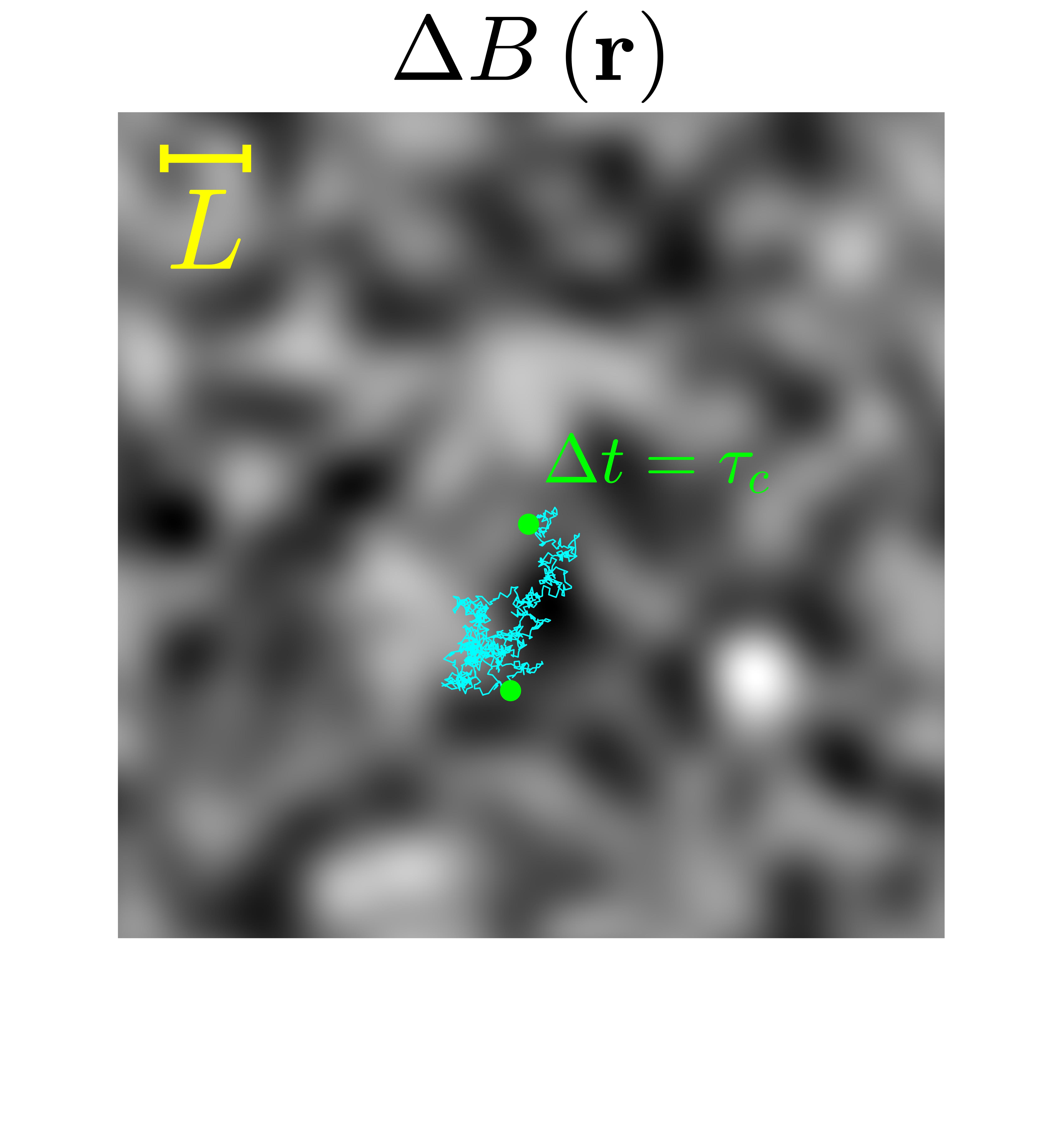
Figure 1: 2D schematic of magnetic field perturbations $$$\Delta B\left(\mathbf{r}\right)$$$ consisting of spatially-correlated Gaussian-distributed noise. The correlation length $$$L$$$ is indicated by the yellow bar. Spins are assumed to diffuse freely through the field, as illustrated by the blue trajectory, which shows the path taken by a representative spin over a time interval $$$\Delta t$$$ equal to the correlation time $$$\tau_c=L^2/D$$$. Note that the 2D representation shown here is for illustrative purposes only; all calculations were performed for a 3D model.
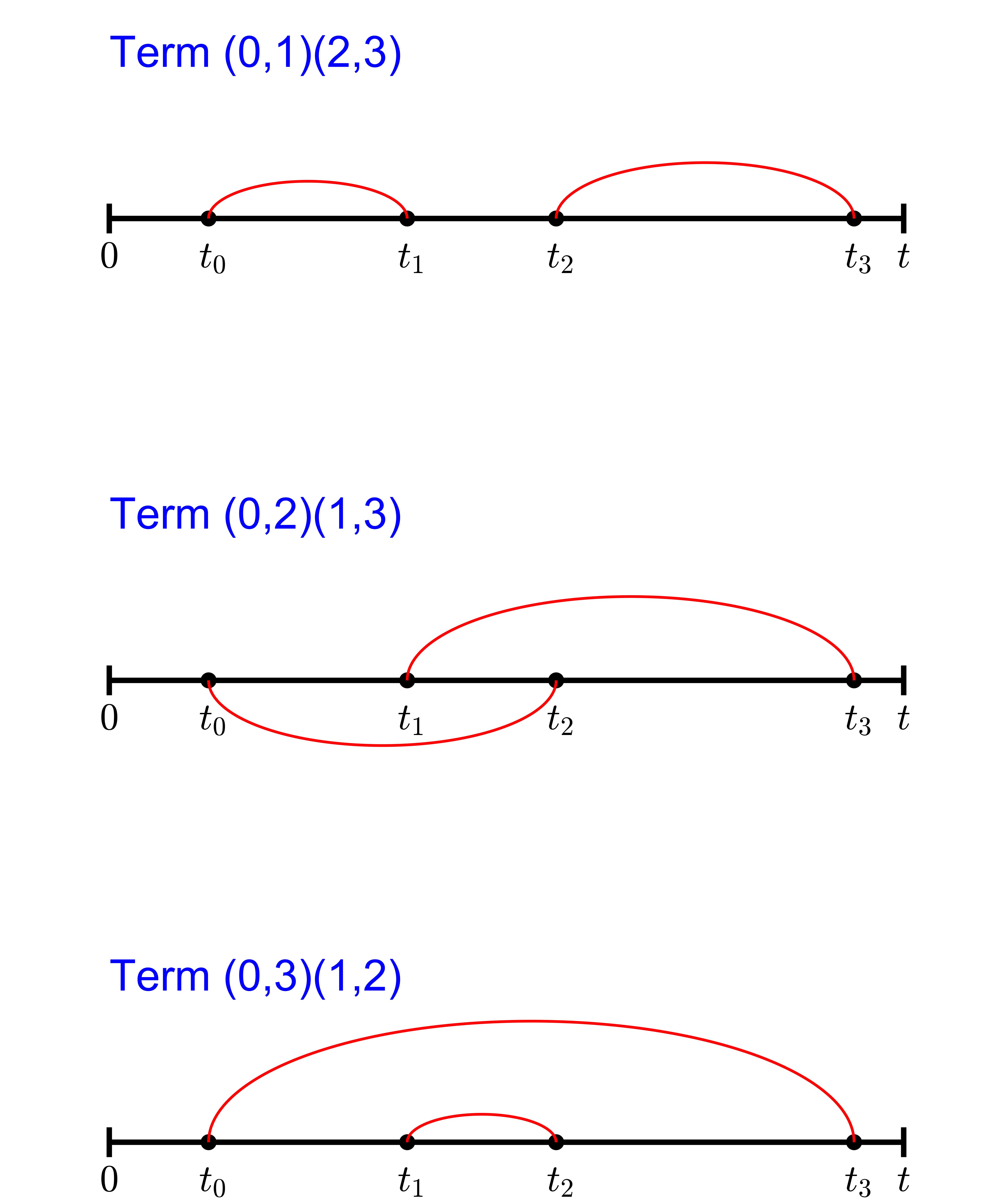
Figure 2: Diagrams illustrating the pairs of points between which field correlations enter into the calculations of the fourth moment, $$$\langle\phi^4(t)\rangle$$$, and the variance squared, $$$\langle\phi^2(t)\rangle^2$$$. Note that the contributions to $$$\langle\phi^4(t)\rangle$$$ and $$$3\langle\phi^2(t)\rangle^2$$$ from the first diagram, $$$(0,1)(2,3)$$$, are identical, and thus cancel in the expression for the fourth-order cumulant, $$$\kappa_4(t)=\langle\phi^4(t)\rangle-3\langle\phi^2(t)\rangle^2$$$.
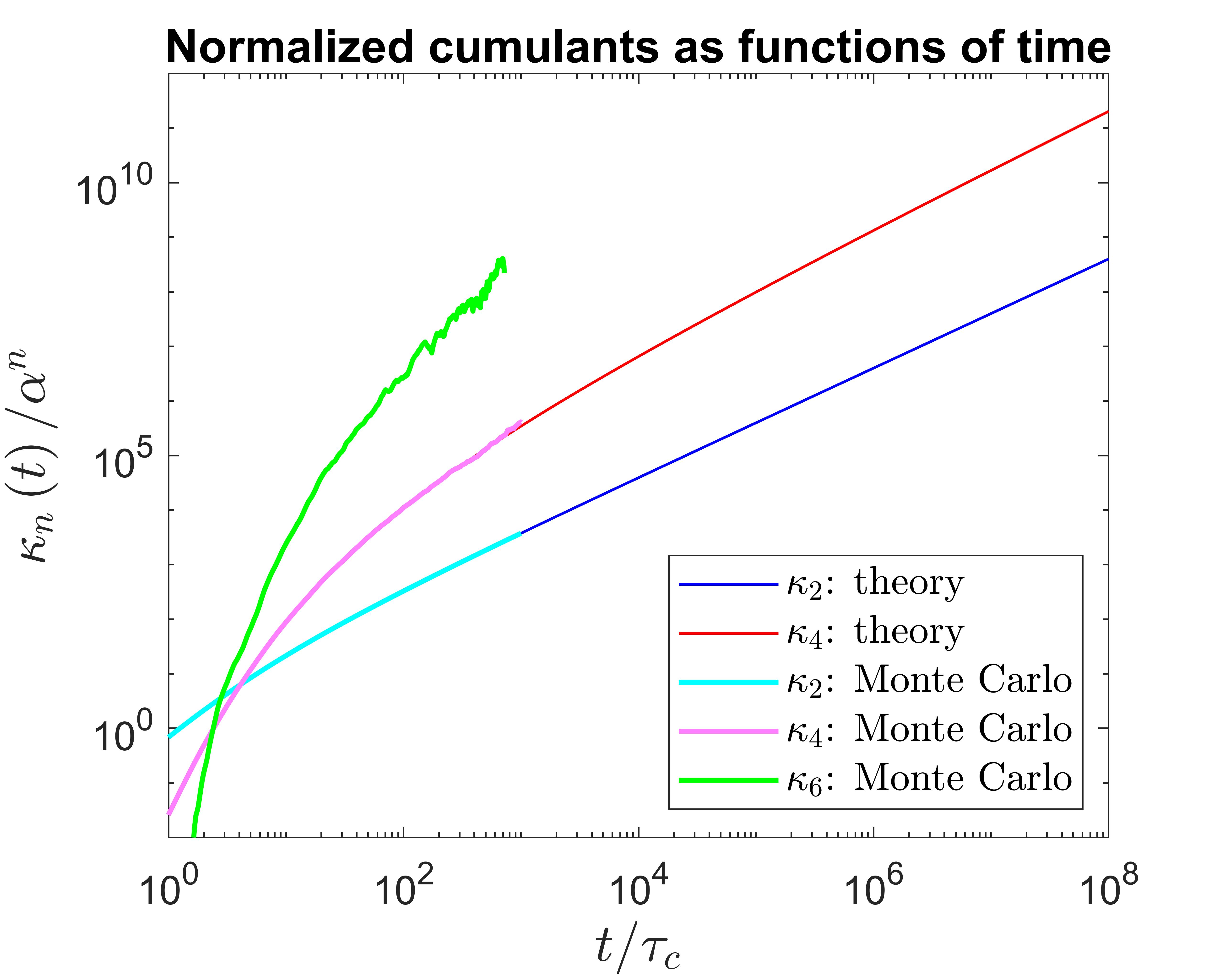
Figure 3: Log-log plot of the first few even-order cumulants as functions of time. The values computed from the integral expressions in the theory section agree well with Monte Carlo results. Each cumulant $$$\kappa_n$$$ is normalized by $$$\alpha^n$$$, where $$$\alpha=\delta\Omega\,\tau_c$$$ represents the amount of dephasing over an interval $$$\tau_c$$$, and quantifies the strength of the signal perturbations. Note that $$$\kappa_4/\alpha^4$$$ exceeds $$$\kappa_2/\alpha^2$$$ after only a few multiples of $$$\tau_c$$$ and continues to increase more rapidly with time.
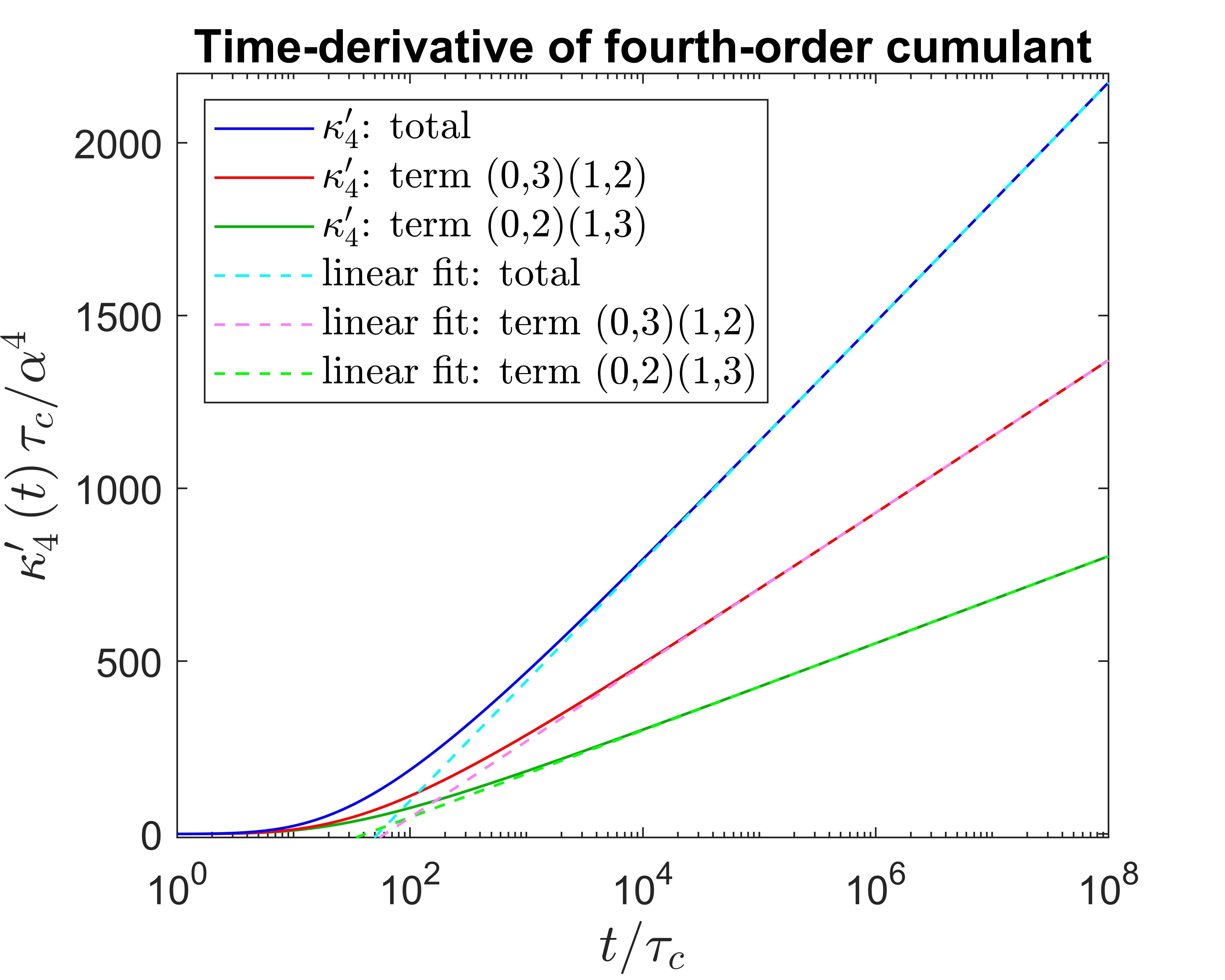
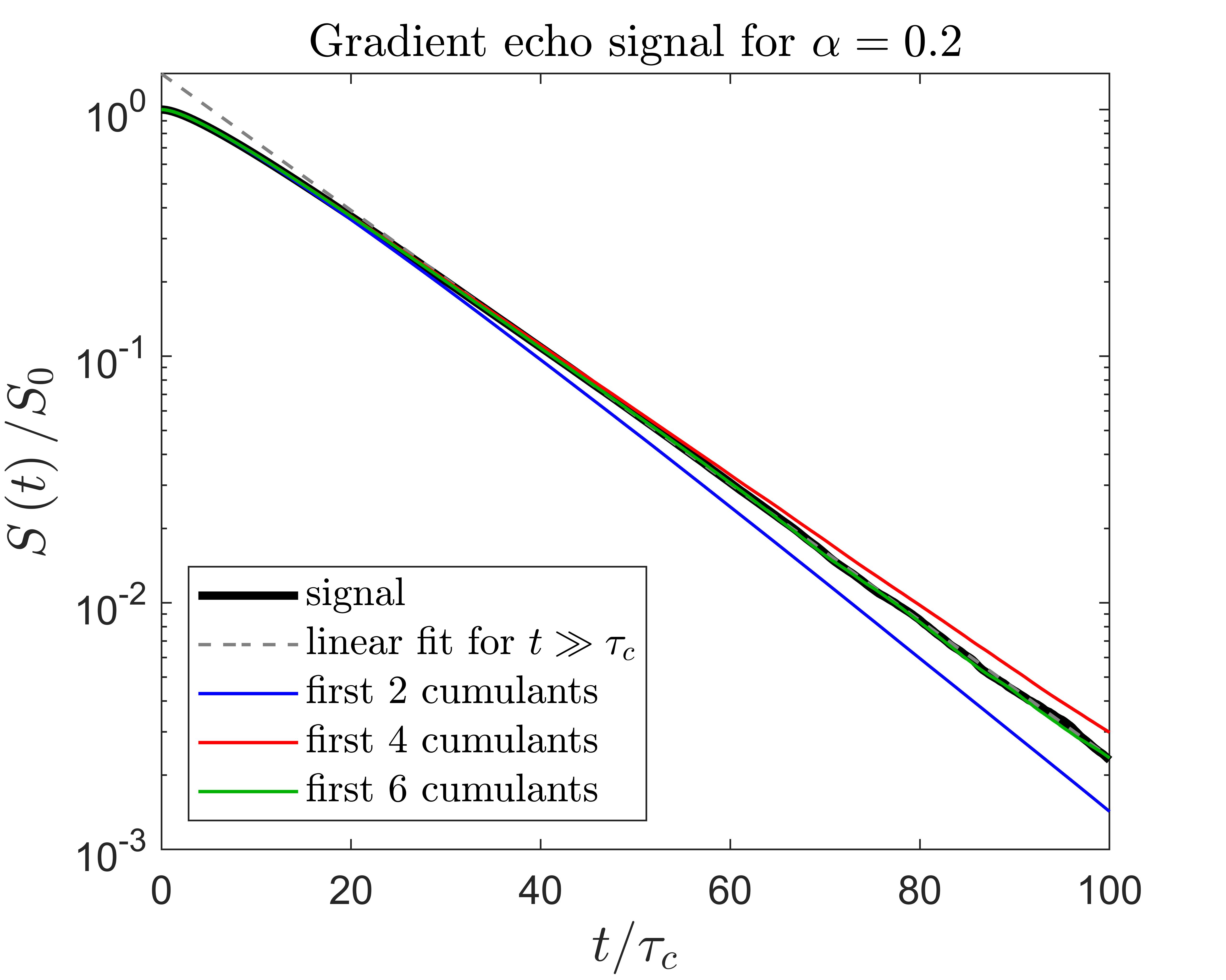
Figure 5: Log-linear plot of the signal, estimated from Monte Carlo simulations. For $$$t\sim\tau_c$$$, the logarithm of the signal exhibits the concave-down signature of microstructure. For $$$t\gg\tau_c$$$, it is well approximated by a straight line, indicative of monoexponential signal decay. The colored curves show cumulant expansions with progressively more terms. Using only $$$\kappa_2(t)$$$ causes substantial undershoot for $$$t\gg\tau_c$$$. Including $$$\kappa_4(t)$$$ slightly overcompensates. Further addition of $$$\kappa_6(t)$$$ provides the best fit.