Synopsis

Keywords: Signal Modeling, Microstructure

In this study, we proposed Bayesian estimation of tissue microstructures in t_d-dMRI model, and compared its performance with the traditional non-linear least square fitting method in simulation data and glioma patient data. We found that the performance of Bayesian fitting was dependent on the prior distribution and choice of hyperparameters, and the combination of Bayesian and least-square fitting could achieve reasonable performance without prior information.

Introduction

Diffusion-time-dependent diffusion MRI ($$$t_d$$$-dMRI) has shown to be useful in mapping cellular microstructures based on dMRI signals acquired at varying $$$t_d$$$, which are fitted with multi-compartment models such as VERDICT^1,2, POMACE³, and IMPULSED^4,5 have been proposed. Due to the highly complex and nonlinear formulation as well as the limited t-space data, fitting of these models were instable and subject to noise using the nonlinear least square fitting approach. This study proposed to use an Bayesian approach to improve microstructural fitting, and test Bayesian fitting with different priors in the IMPULSED model on both simulated data and pediatric glioma data.

Methods

$$$t_d$$$-dMRI model:
In the IMPLSED framework, tissues were characterized by a two-compartment model based on dMRI measured in the short-to-median $$$t_d$$$ regime with oscillating or pulsed gradient sequences. The total decay could be represented as contributions from both intracellular and extracellular space, according to the $$$t_d$$$-dependent analytical formulation for impermeable spheres⁴.

$$ \frac{S(g)}{S(0)}=A(f_{in},d,D_{ex})=f_{in} S_{in} (d,D_{in},δ,Δ,g,t_r,f)+(1-f_{in})S_{ex} (D_{ex},g)$$

where $$$S_{in}$$$ and $$$S_{ex}$$$ represent intracellular and extracellular signals respectively⁶. The intracellular fraction $$$f_{in}$$$, cell diameter $$$d$$$, and extracellular diffusion coefficient $$$D_{ex}$$$ are the microstructure parameters to be estimated, and $$$D_{in}$$$ was fixed at 1 μm²/ms in this study according to⁶.

Bayesian fitting:
In the Bayesian framework, the posterior probabilities of microstructural parameters could be presented as the product of likelihood functions and prior probabilities:
$$P(f_{in},d,D_{ex} |\frac{S(g)}{S(0)} )∝P(\frac{S(g)}{S(0)} |f_{in},d,D_{ex}) \cdot P(f_{in},d,D_{ex})$$
The posterior distributions were estimated using a Markov chain Monte Carlo (MCMC) setup based on Gibbs sampling and the Metropolis-Hastings algorithm⁷.
Assuming white Gaussian noise, the marginal likelihood function could be obtained by integrating the noise variance⁸:
$$P( \frac{S(g)}{S(0)} │f_{in},d,D_{ex} )∝\left[\frac{1}{2} \sum_{i=1}^n\left(\frac{S_i}{S_0} -A(f_{in},d,D_{ex})\right)^2 \right]^{-\frac{n}{2}}$$
Where $$$n$$$ is the number of measured dMRI signals, and $$$A$$$ is IMPULSED model. We set the prior probability distributions of $$$f_{in}$$$ and $$$D_{ex}$$$ to be uniform, and four types of priors were tested for cell diameter $$$d$$$, including
(1) uniform :
$$P(d)∝1$$
(2) reciprocal:
$$P(d)∝\frac{1}{d}$$
(3) Gaussian:
$$P(d|μ,σ)=\frac{1}{σ\sqrt{2π}} e^{⁡-\frac{(d-μ)^2}{2σ^2 }}$$
(4) lognormal distribution:
$$P(d|μ,σ)=\frac{1}{dσ\sqrt{2π}} e^{⁡-\frac{(ln⁡d-μ)^2}{2σ^2 }}$$
where the expectation and variance of the lognormal distribution are: $$E(d)=e^{μ+\frac{σ^2}{2}}\qquad$$
$$D(d)=(e^{σ^2 }-1)e^{2μ+σ^2}$$
The Bayesian fitting results were compared with nonlinear least square (NLLS) fitting. The fitting was repeated 100 times with randomly generated initial values, and the result with smallest fitting residual were chosen as the final results. The prior distribution of Bayesian estimation was set using the results from NLLS fitting , e.g., $$$μ;E(d)=d_{NLLS} $$$ and $$$σ;D(d)=10;80$$$ for Gaussian or lognormal distribution respectively.

Simulation experiment:
Simulated signals were generated according IMPULSED model, and white Gaussian noise with SNR=80 was added. The parameter space $$$(f_{in},d,D_{ex})$$$ was sampled at $$$f_{in}=0.01-0.6 $$$ with a step size 0.01,$$$d=5-30$$$μm with a step size 0.1 μm, and $$$D_{ex}=1-2$$$μm²/ms with a step size 0.01 μm²/ms, resulting in a total of 40,000 samples.


Glioma data acquisition:
The pediatric glioma were acquired on a 3T Phillps scanner with house-made oscillating and pulsed gradient dMRI sequences from 49 high-grade and 20 low-grade gliomas⁹. The acquisition protocols were as follows:$$$δ=60ms,Δ=82.3ms,t_r=1.6ms$$$, $$$b=500,1000,2000 s/mm²$$$ for PGSE and OGSE($$$f=17Hz$$$),$$$b=500 s/mm²$$$ for OGSE($$$f=33Hz$$$),$$$b=350 s/mm²$$$ for OGSE($$$f=50Hz$$$). 6 diffusion directions per b-value, TE/TR=168/3000 ms , FOV = 180×180 mm², in-plane resolution=1.41×1.41 mm², 3 slices with thickness of 8 mm.

Results

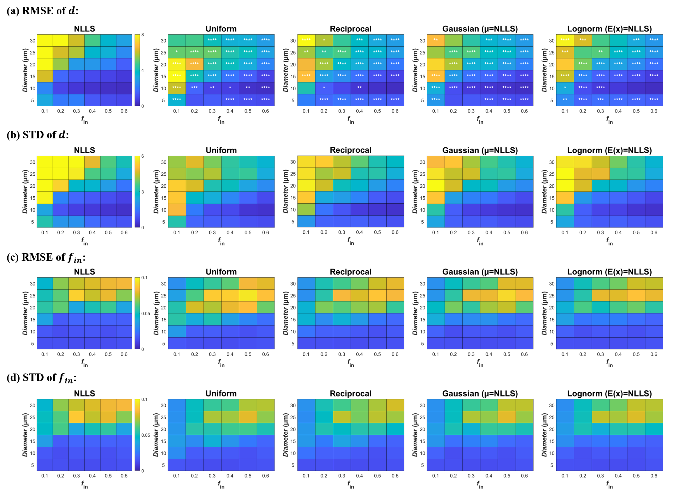
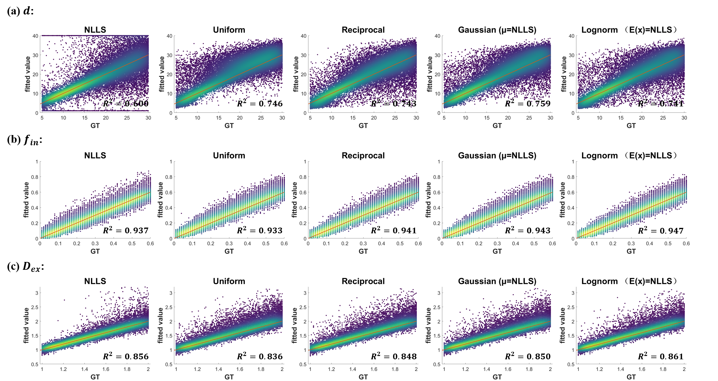
The simulation experiment showed that NLLS method resulted in a large variation in the estimated cell diameter $$$d$$$ according to the standard deviation (STD) of the fitted values, and the error was particularly large with low $$$f_in$$$ and high $$$d$$$ (upper left portion of Fig. 1 heatmap) based on the root mean square error (RMSE) compared to the ground truth. The use of Bayesian estimation considerably reduced the variation, and the fitting errors were significantly reduced (as indicated by the significance levels). Different prior distributions led to slight differences in the estimation of $$$d$$$ but not on $$$f_in$$$, and the variation was the lowest using Gaussian and lognormal distributions (Fig. 2).
Correlation plots between estimated values and groundtruth in Fig. 2 showed the estimated $$$d$$$ using NLLS method often approached the fitting boundary (1 or 40μm), which can be avoided by the Bayesian estimation. Uniform and reciprocal distributions corrected the off-diagonal values toward the center (Fig.2) . The combination of NLLS and Bayesian estimation improved linear correlation between estimated values and ground truth (Table 1). Table 1 also showed that the RMSE and STD for $$$d$$$ was significantly reduced using the Bayesian method compared with NLLS. For $$$f_{in}$$$ and $$$D_{ex}$$$, NLLS and Bayesian fitting showed equivalent performance, possibly because the estimation of $$$f_{in}$$$ and $$$D_{ex}$$$ was already good with NLLS.
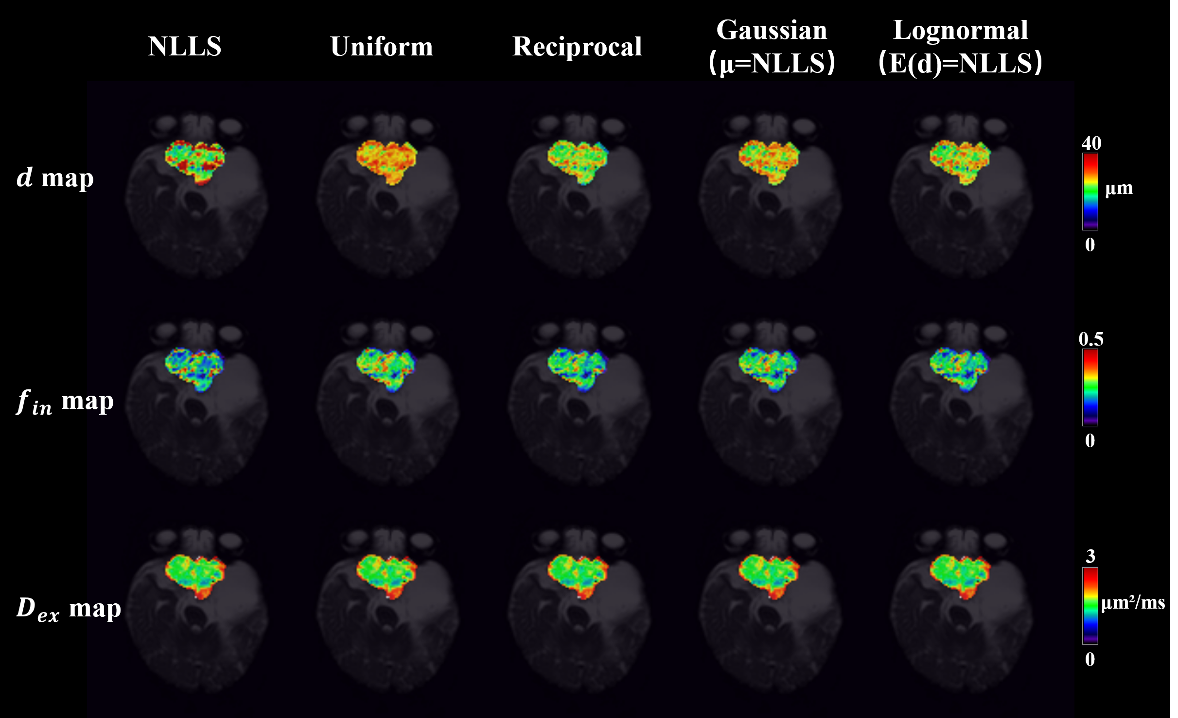
The microstructural map of pediatric glioma (Fig.3) demonstrated reduced variation and erroneous fitting in $$$d$$$. Diagnostic analysis of the 69 patients (Table 2) indicated that $$$f_{in}$$$ had the highest AUC in differentiating high- and low-grade glioma, and the use of Bayesian method further improved AUC compared to NLLS.

Discussion and Conclusion

We found that Bayesian estimation improve the fitting accuracy and stability, especially for the estimation of d in the IMPULSED model. The choice of prior distribution played a significant role in IMPULSED model fitting.In the absence of prior information, the combination of NLLS and Bayesian estimation could better improve the estimation effect of cell diameter $$$d$$$.

Acknowledgements

This work is supported by Ministry of Science and Technology of the People’s Republic of China (2018YFE0114600, 2021ZD0200202), National Natural Science Foundation of China (61801424, 81971606, 82122032), and Science and Technology Department of Zhejiang Province (202006140, 2022C03057).