4250
SNR Visualization: A Toolbox for Locating Flexible Coil Arrays
Pulkit Malik1, Tracy Wynn1, Peter Fischer1, and Gillian Haemer1
1InkSpace Imaging, Pleasanton, CA, United States
1InkSpace Imaging, Pleasanton, CA, United States
Synopsis
Keywords: RF Arrays & Systems, Data Analysis, Receive Array SNR
We present a MATLAB based visualization toolbox for locating coil elements and evaluating SNR for flexible coil arrays. The greater variation in coil positioning creates challenges for SNR comparisons. By locating coils with coil sensitivity isocontours, the SNR of individual channels can be evaluated while the coil array is flexed. This is used to examine the repeatability of placement, and changes to coil coupling in the different placements. The coil locations can be validated using the SNR visualization displayed as slices, lines, and probe points. Expectations of the SNR field shape are used to further optimize coil locations.Introduction
Signal to noise characterization of receive arrays is an important foundation for coil development and analysis. Flexible receive arrays have received increased interest for their subject-specific adaptability, patient-friendliness, and clinical usability1-8. However, repeatable, quantitative SNR characterization can be challenging. Changes in individual element positions relative to the subject create a data registration issue, often mitigated with the use of custom fixturing or registration algorithms. Because flexible coils are intended to conform to patient anatomy, positioning the coil around the subject often results in variations in coil loading and coupling, information which is lost by using one-size fits all fixtures. In this work we present an SNR toolbox which uses coil sensitivity mapping to inform the user on coil positioning and loading, and which generates individual element SNR measurements. This toolbox allows for SNR comparison on an individual element basis, while generating a visual representation of element positions relative to the subject.Method
SNR for was first measured on a 3T scanner by acquiring a 3D spoiled gradient echo (TR/TE/FA/BW/Res = 140ms/3ms/30°/62.5Hz/[1.25,1.25,2] mm), and an equivalent noise scan without RF excitation. The data was analyzed in Matlab (2019A) using the Kellman method9 to output a 3D matrix in SNR units. The coil images and SNR matrix were used as the input to the toolbox for SNR visualization and coil position analysis.Coil locations were calculated using sensitivity isocontours to estimate a vector normal to the coil. Centroids of the 3D isocontours were used to perform a linear regression. The resulting unit vector was used to determine the tilt of the coil, and the coil was located based on a user-chosen distance from the first isocontour.
After the automated calculation, the toolbox allows manual adjustment of coil rotation and offset distance. Individual element SNR is proportional to field strength and falls off relative to the distance from the coil, so it may be analyzed according to the following equation, where R is the coil radius and y is the distance to the coil:
$$\vec{B} = \frac{\mu_0 I R^2}{2(y^2 + R^2)^{3/2}}\hat{\mathit{j}}$$
By evaluating SNR along the normal vector relative to the equation above, the position and angle of the vector may be optimized to best suit the data, including a global correction for B1 twist.
After coil positions, normal vectors, and isocontour plots have been calculated, the visualization is generated. The combined SNR image is visualized in 3-dimensions using 2D sagittal, coronal, and axial slices. Slice positions can be adjusted to visualize the entire volume. SNR line profiles along plane intersections are plotted to visualize the overall shape and level of SNR through the phantom. Finally, for each coil a probe into the volume along the normal vectors is shown and used to calculate a point SNR measurement at a given depth to provide quantitative measurements for each channel. Isocontour plots can be displayed within the visualization and may be used to optimize coil locations and compensate for B1 twist (LISA artifact).
Discussion
SNR comparisons of flexible coils are often performed on flat phantoms to minimize variations in coupling between elements and in coil loading, and to allow for easy analysis of SNR in a 2D slice at a set distance from the array. However, variations in coupling and loading based on positioning is an intrinsic part of a flexible coil’s SNR that should be captured in analysis, and evaluating coils in a wrapped geometry for various applications is often important. The purpose of this SNR toolbox is to effectively compare SNR of flexible coils in representative positions for varying use cases. By locating and visualizing individual elements’ SNR, we hope to move closer to a quantitative and fair comparison tool between flexible coils and non-flexible industry standard arrays, taking loading and coil positioning into account.Further refinement of this toolbox is in progress to make it a more powerful tool. First, the visualization tool currently uses a sum-of-squares based SNR calculation. Adding a more complex SNR processing tool to utilize coil sensitivity maps may improve analysis of coil coupling. Second, manual adjustment of the normal vector for individual elements relative to the expected profile will be upgraded to include a gradient descent aided optimization to improve usability. Third, automated calculations of B1 twist, based on known properties will be included to improve coil visualization. Finally, phase maps of the coil array generated via the body coil could provide detailed information about coil orientation.
Conclusion
This toolbox is still in the early stages of development, yet it has already been useful in identifying global variations in coil positioning. Day-to-day variations in coil positioning have been confirmed by the automated coil position visualization of the SNR. As the toolbox is used and updated, we expect to minimize variation in SNR measurements between setups for our flexible arrays.Acknowledgements
This work was supported in part by NIH grant R44 EB028728-03.References
[1] Nordmeyer-Massner, et al; MRM 2009. 61(2):429-38.
[2] Corea, et al; Nat Commun 2016. 7: 10839.
[3] Rossman, et al; ISMRM 2017: p763.
[4] Frass-Kriegl, et al; PLoS One 2018. 13(11): e0206963
[5] McGee, et al; Phys Med Biol 2018. 63(8): 08NT02.
[6] Zhang, et al; Nature Biomed Eng 2018. 2(8): 570-7.
[7] Zhang, et al; MRM 2019. 81(5): 3406-15.
[8] Collick, et al; Phys Med Biol 2020. 65(19): 19NT01.
[9] Darnell, et al; JMRI 2021. 55(4): 1026-42.
[9] Kellman, et al; MRM, 2005. 54(6): 1439-47.
Figures
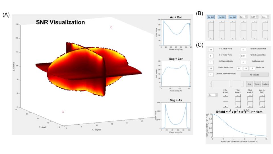
The toolbox displays three windows. A) The SNR
visualization window displays a 3D image volume of the SNR as sliced planes. To
the right, line graphs show 1D intersections of the slices. Values associated
with vector probes can be toggled to display at the bottom. B) The SNR and
channel map plots scrollers control the slice positions. C) In this window parameter
definitions are used to calculate coil locations, and manual adjustment tools are
used optimize coil positions. The plot at the bottom of
the window shows expected and calculated centerline SNR for a channel.
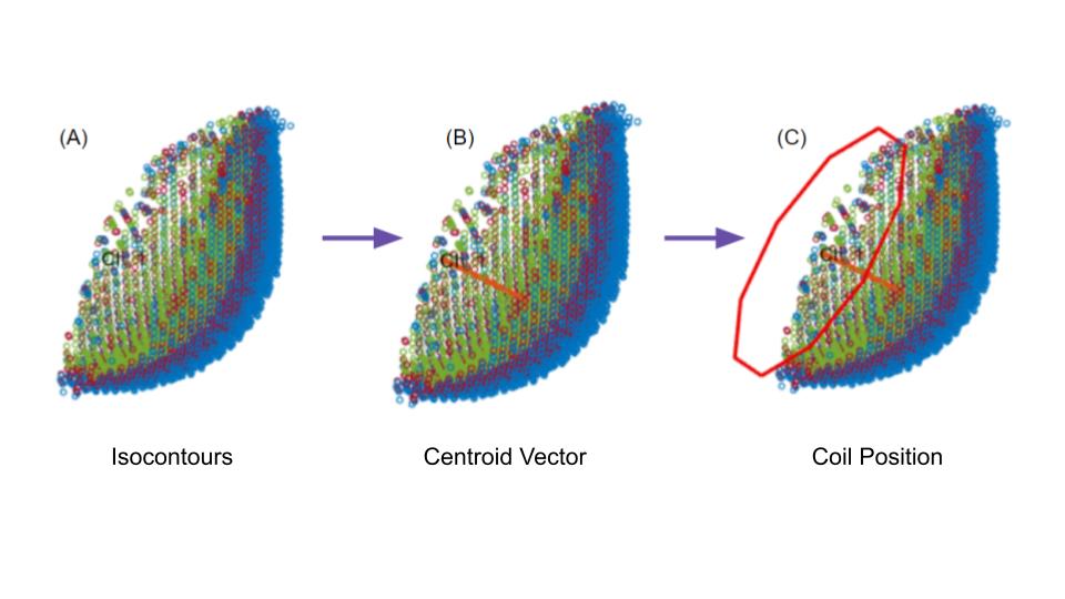
Each coil position is initially estimated
using a normal vector created by the centroids of the sensitivity map
isocontours. User specified percentiles of the sensitivity maps are used to
determine the isocontours (A). Centroids of each isocontour are used to perform
a linear regression to determine the vector normal to the expected coil angle
(B, vector shown in red). The resulting unit vector is used to visualize the
expected coil position (C) at a user specified distance from the phantom. The parameters
can be adjusted by the user to better match the expected coil distribution.
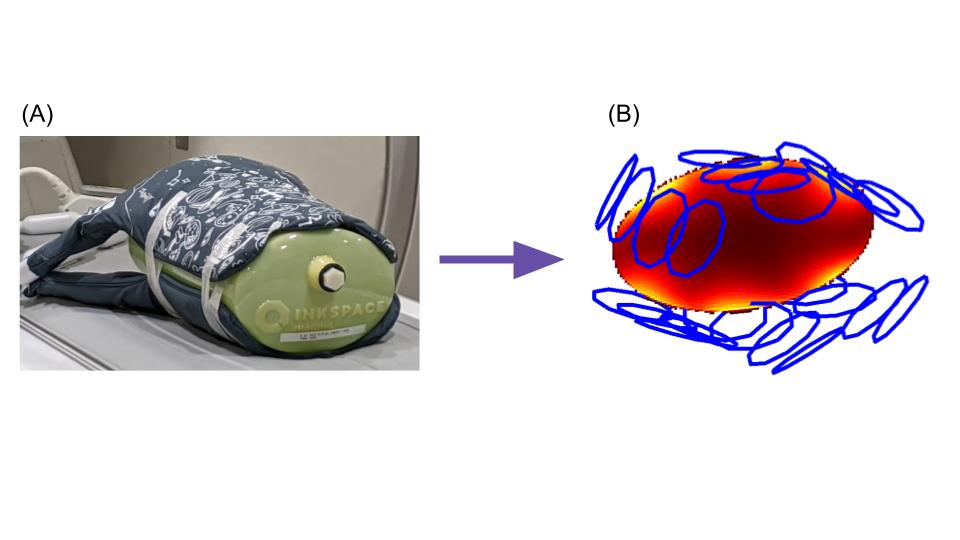
Example visualization of a commercial flexible
array (InkSpace Imaging Pediatric Body Array). The coil is wrapped tightly
around a large cylindrical phantom (A). The curved geometry of the coil and the
phantom are visualized in the initial coil position estimate (B). The initial
coil map is shown with calculated SNR in the phantom through a single axial
slice. Though some errors in the coil angles remain in the automated calculation,
these can be improved by a manual adjustment.
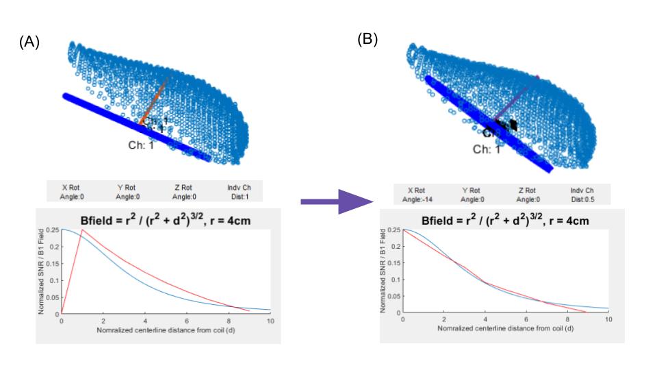
Coil positions
can be adjusted by adding to the x, y, or z axis rotations, or the offset
distance from the phantom (controls in Figure 1C). Users can make an educated
adjustment based on the isocontour plots and the expected shape of the B1 Field
through the centerline of the coil. An automated coil position (A), is optimized
manually by adjusting both the x-axis rotation and the coil offset to ensure
the SNR falloff and the expected B1 field are aligned (B). Matching the vector
and shape yields a coil position which appears closer to an expected position
based on SNR distribution.
DOI: https://doi.org/10.58530/2023/4250