4247
Quasi-Static and Time-Generalized Field Computation Methods Compared to the Moment Method for Performance Evaluations of Coil Arrays in PI at UHF1Institute of Medical Physics and Radiation Protection, TH Mittelhessen University of Applied Science, Giessen, Germany
Synopsis
Keywords: RF Arrays & Systems, Parallel Imaging, Phased Array, Electromagnetic Field Simulations
In this study, we compared the quasi-static method (QSM), the time-generalized method (TGM), and the method of moments (MoM) for performance evaluations of coil arrays in parallel imaging (PI) at UHF. We have shown that the QSM and the TGM are a good approximation to the MoM solution, and that all three methods perform similarly in a comparative study with a 64-channel head coil. Furthermore, we could show, that the TGM performs better than the QSM at larger distances in the phantom, which may be beneficial for the evaluation of torso coils.
Introduction
The SNR and the g-factor of coil arrays used in parallel imaging (PI) depends strongly on the geometrical arrangement of the coil and the reception profiles of each element in the array1-4. According to the principle of reciprocity5, the complex reception profile of a receiving coil can be expressed by the transversal magnetic field, generated when a current flows through the coil. Similarly, the intrinsic correlation between the noise in various elements of an array can be expressed in terms of electric fields6. Consequently, many methods have been proposed for field computations in MRI7. In this study, we compared the Quasi-Static, Time-Generalized, and the Moment-Method for coil performance evaluations in PI at UHF.Theory
Quasi-Static Method (QSM): The vector potential for the quasi-satic case is given by8-11\begin{equation}\mathbf{A}(\mathbf{r})=\frac{\mu}{4\pi}\int\frac{Id\mathbf{r}'}{|\mathbf{r}-\mathbf{r}'|}.\qquad(1)\end{equation}With the well known relations\begin{align}\mathbf{E}&=-\frac{\partial}{\partial t}\mathbf{A}=-j\omega\mathbf{A},\qquad(2)\\\mathbf{B}&=\nabla\times\mathbf{A},\qquad(3)\end{align}we obtain the following expressions\begin{align}\mathbf{E}(\mathbf{r})&=-\frac{j\omega\mu}{4\pi}\int\frac{Id\mathbf{r}'}{|\mathbf{r}-\mathbf{r}'|},\qquad(4)\\\mathbf{B}(\mathbf{r})&=\frac{\mu I}{4\pi}\int\frac{d\mathbf{r}'\times\mathbf{r_u}}{|\mathbf{r}-\mathbf{r}'|^2}.\qquad(5)\end{align}Here, $$$I=1\,A$$$ is the unit current, $$$\mathbf{r}$$$ the observation point, $$$\mathbf{r}'$$$ the source point, $$$\mathbf{r_u}$$$ the unit vector in direction of $$$|\mathbf{r}-\mathbf{r}'|$$$, $$$j=\sqrt{-1}$$$ the imaginary unit, and $$$\omega$$$ the angular frequency.Time-Generalized Method (TGM): If we assume a time-harmonic dependence $$$exp(+j\omega t)$$$ the vector potential is given by12-15\begin{equation}\mathbf{A}(\mathbf{r})=\frac{\mu}{4\pi}\int\frac{\mathbf{J}(\mathbf{r}')}{|\mathbf{r}-\mathbf{r}'|}\exp(-jk|\mathbf{r}-\mathbf{r}'|) d^3r',\qquad(6)\end{equation}where $$$\mathbf{J}(\mathbf{r}')$$$ is the current density and $$$k$$$ the wave number for an absorbing medium:\begin{equation}k=\alpha+j\beta=\omega\sqrt{\mu_0\mu_r\epsilon_0(\epsilon_r+\frac{\sigma}{j\omega\epsilon_0})}.\qquad(7)\end{equation}Using equations (2-3) and the vector identity\begin{equation}\nabla\times(\psi\mathbf{A})=\nabla\psi\times\mathbf{A}+\psi\nabla\times\mathbf{A}\qquad(8)\end{equation}we obtain16-17\begin{align}\mathbf{E}(\mathbf{r})&=-\frac{j\omega\mu}{4\pi}\int\frac{\mathbf{J}(\mathbf{r}')}{|\mathbf{r}-\mathbf{r}'|}\exp(-jk|\mathbf{r}-\mathbf{r}'|)d^3r',\qquad(9)\\\mathbf{B}(\mathbf{r})&=\frac{\mu}{4\pi}\int\left[\frac{\mathbf{J}(\mathbf{r}')}{|\mathbf{r}-\mathbf{r}'|^2}+jk\frac{\mathbf{J}(\mathbf{r}')}{|\mathbf{r}-\mathbf{r}'|}\right]\exp(-jk|\mathbf{r}-\mathbf{r}'|)\times\mathbf{r_u}d^3r.\qquad(10)\end{align}For a filamentary current ($$$\mathbf{J}(\mathbf{r}')d^3r=I(\mathbf{r}')d\mathbf{r}'$$$) we can also write\begin{align}\mathbf{E}(\mathbf{r})&=-\frac{j\omega\mu}{4\pi}\int\frac{I(\mathbf{r}')}{|\mathbf{r}-\mathbf{r}'|}\exp(-jk|\mathbf{r}-\mathbf{r}'|)d\mathbf{r}',\qquad(11)\\\mathbf{B}(\mathbf{r})&=-\frac{\mu}{4\pi}\int\left[\frac{I(\mathbf{r}')}{|\mathbf{r}-\mathbf{r}'|^2}+jk\frac{I(\mathbf{r}')}{|\mathbf{r}-\mathbf{r}'|}\right]\exp(-jk|\mathbf{r}-\mathbf{r}'|)\mathbf{r_u}\times d\mathbf{r}'.\qquad(12)\end{align}For simplicity, we assume that $$$I(\mathbf{r}')$$$ is uniformly distributed $$$(I=1\,A)$$$ and time-harmonic. Method of Moments (MoM): The electric field intensity in an arbitrarily-shaped, inhomogeneous dielectric body can be expressed as a superposition of two fields18\begin{equation}\mathbf{E}(\mathbf{r})=\mathbf{E}^{ex}(\mathbf{r})+\mathbf{E}^{eq}(\mathbf{r}),\qquad(13)\end{equation}where the fields are given by\begin{align}\mathbf{E}^{ex}(\mathbf{r})&=(k_0^2+\nabla\nabla\cdot)\mathbf{A}^{ex}(\mathbf{r}),\qquad(14)\\\mathbf{E}^{eq}(\mathbf{r})&=(k_0^2+\nabla\nabla\cdot)\mathbf{A}^{eq}(\mathbf{r}),\qquad(15)\end{align}and the vector potentials by\begin{align}\mathbf{A}^{ex}(\mathbf{r})&=\frac{j}{\omega\epsilon_0}\int G(\mathbf{r},\mathbf{r}')\mathbf{J}^{ex}(\mathbf{r}')d^3r,\qquad(16)\\\mathbf{A}^{eq}(\mathbf{r})&=\frac{j}{\omega\epsilon_0}\int G(\mathbf{r},\mathbf{r}')\mathbf{J}^{eq}(\mathbf{r}')d^3r,\qquad(17)\end{align}in which $$$G(\mathbf{r},\mathbf{r}')$$$ is the free-space Green's function\begin{equation}G(\mathbf{r},\mathbf{r}')=\frac{\exp(jk_0|\mathbf{r}-\mathbf{r}'|)}{4\pi|\mathbf{r}-\mathbf{r}'|}.\qquad(18)\end{equation}$$$\mathbf{J}^{ex}$$$ is the excitation current and $$$\mathbf{J}^{eq}=-j\omega\epsilon_0(\epsilon_c-1)\mathbf{E}(\mathbf{r})$$$ the volumetric equivalent current, which accounts for the dielectric and conductive effects of the inhomogeneous body. The magnetic flux density can also be expressed as a superposition of two fields\begin{equation}\mathbf{B}(\mathbf{r})=\mathbf{B}^{ex}(\mathbf{r})+\mathbf{B}^{eq}(\mathbf{r}),\qquad(19)\end{equation}where the fields are given by\begin{align}\mathbf{B}^{ex}(\mathbf{r})&=-j\omega\epsilon_0\mu\nabla\times\mathbf{A}^{ex}(\mathbf{r}),\qquad(20)\\\mathbf{B}^{eq}(\mathbf{r})&=-j\omega\epsilon_0\mu\nabla\times\mathbf{A}^{eq}(\mathbf{r}).\qquad(21)\end{align}These equations are usually discretized using the Galerkin method, resulting in matrix equations that provides a numerical solution to the electromagnetic problem.Simulations
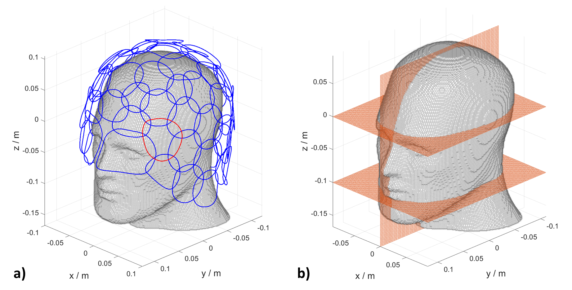
We calculated $$$\mathbf{E}$$$ and $$$\mathbf{B}_1$$$ for a 64-channel coil array (Fig.1) loaded with a human head model ($$$\epsilon_r=52,\;\sigma=0.55\,S/m$$$) using the QSM (Eqs.4-5) and the TGM (Eqs.11-12) at 7T. To obtain the MoM-solution, we used the integral equation solver MARIE19-21. In addition, we computed the resulting reception profiles ($$$B_1^-$$$) using each method and evaluated the coil in terms of noise correlation, SNR, and g-factor. For this we used the following formulas:\begin{align}&C=B_1^-=\frac{1}{2}(B_x-jB_y)^*,\qquad(22)\\&\Psi_{ij}=\int\sigma(\mathbf{r})\mathbf{E}_i\cdot\mathbf{E}^*_jd^3r,\qquad(23)\\&\Psi^{cor}_{ij}=\frac{\Psi_{ij}}{\sqrt{\Psi_{ii}\Psi_{jj}}},\qquad(24)\\&SNR=\sqrt{C^H\Psi^{-1}C},\qquad(25)\\&g_p=\sqrt{[(C^H\Psi^{-1}C]^{-1}]_{pp}^{red}C^H\Psi^{-1}C]_{pp}^{red}}.\qquad(26)\end{align}
Results and Discussion
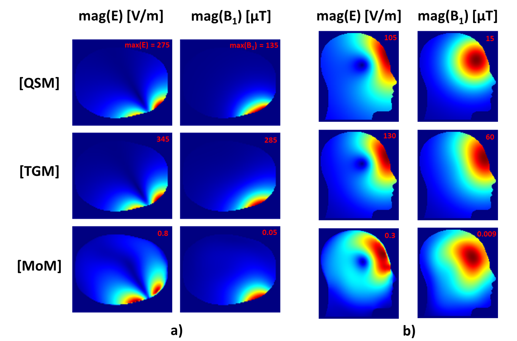
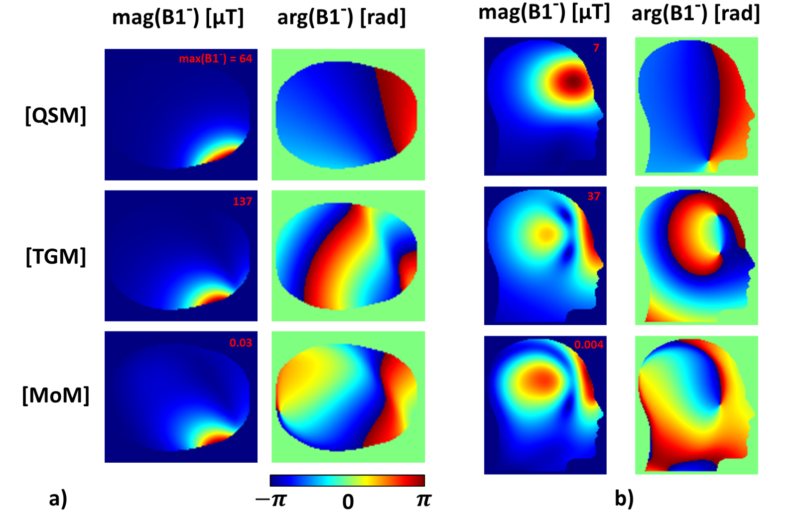
Figures 2 and 3 shows the magnitude-plots of the fields $$$\mathbf{E}$$$, $$$\mathbf{B}_1$$$, and $$$B_1^-$$$ generated by the red coil in Fig.1, calculated using the QSM, TGM, and MoM, respectively. Figure 3 shows the phases of the $$$B_1^-$$$ fields as well. It can be observed that all methods provide magnitude plots that are in good overall agreement. However, the TGM provides $$$B_1^-$$$ fields, where field splitting is observed due to the higher frequencies at UHF. This effect is not included in the QSM since the currents flowing through the coils are stationary. It is also observed that in the coil's proximity, the phases obtained with the TGM agree better with the MoM results (with a shift of $$$\pi$$$), while the QSM does not give reliable results, which can be attributed to the missing phase information of the radiative field components.Figure 3a shows the noise correlation $$$\Psi^{cor}$$$ of the coil array calculated by each method. It is obvious that the noise correlation calculated with QSM agrees well with the values obtained with MoM, while the TGM values are significantly lower (QSM: mean=.15,std=.15; TGM: mean=.07,std=.09; MoM: mean=.14,std=.14). Compared to the QSM (Eq.4), the electric field strength (Eq.11) of the TGM contains an additional exponential function $$$exp(-j\cdot imag(k)\cdot|\mathbf{r}-\mathbf{r}'|)$$$, so that the amplitude of the TGM field decreases faster at depth, resulting in a lower value of the volume integral in Eq.23. This effect is also present in the MoM-approach, but the equivalent currents $$$\mathbf{J}^{eq}$$$ lead to additive fields at depth, so that the values of (Eq.23) remain at a high level.
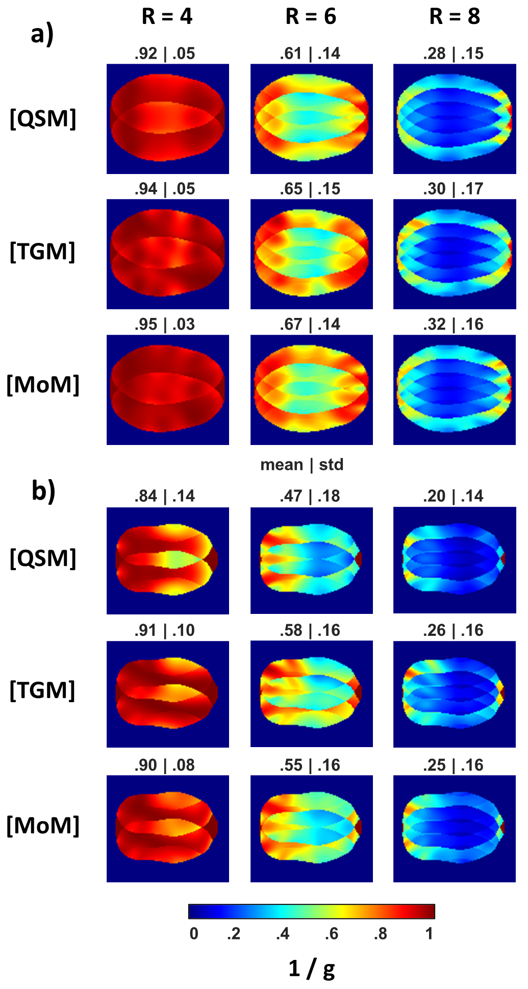
Figure 3b and 4 show the SNR and g-factors (R=4,6,8) of the coil array. The numbers above the plots indicate the mean and standard deviation. In the cortical regions of the head phantom, all methods perform equally well. In the central region, it can be observed that the TGM performs better than the QSM. This can be attributed to the radiation field components ($$$\propto1/|\mathbf{r}-\mathbf{r}'|$$$), which are present in the TGM and MoM but missing in the QSM.
Conclusion
All three methods perform similarly in the head coil study shown. The TGM performs better than the QSM at greater phantom depths, which may be beneficial for evaluating torso coils. We will verify these hypothesis in further studies.Appendix
To obtain Equation (10) we start with\begin{equation}\mathbf{B}(\mathbf{r})=\nabla\times\mathbf{A}(\mathbf{r})=\nabla\times\frac{\mu}{4\pi}\int\mathbf{J}(\mathbf{r}')\frac{\exp(-jk|\mathbf{r}-\mathbf{r}'|)}{|\mathbf{r}-\mathbf{r}'|}d^3r'=\frac{\mu}{4\pi}\int\nabla\times\left[\mathbf{J}(\mathbf{r}')\frac{\exp(-jk|\mathbf{r}-\mathbf{r}'|)}{|\mathbf{r}-\mathbf{r}'|}\right]d^3r'.\end{equation}Using\begin{equation}\nabla\times(\psi\mathbf{A})=\nabla\psi\times\mathbf{A}+\psi\nabla\times\mathbf{A}\end{equation}we get\begin{equation}\mathbf{B}(\mathbf{r})=\frac{\mu}{4\pi}\int\left[\nabla\left(\frac{\exp(-jk|\mathbf{r}-\mathbf{r}'|)}{|\mathbf{r}-\mathbf{r}'|}\right)\times\mathbf{J}(\mathbf{r}')+\frac{\exp(-jk|\mathbf{r}-\mathbf{r}'|)}{|\mathbf{r}-\mathbf{r}'|}\nabla\times\mathbf{J}(\mathbf{r}')\right]d^3r'.\end{equation}Further applies\begin{align}&\nabla\left(\frac{\exp(-jk|\mathbf{r}-\mathbf{r}'|)}{|\mathbf{r}-\mathbf{r}'|}\right)=-\mathbf{r_u}\left(\frac{1+jk|\mathbf{r}-\mathbf{r}'|}{|\mathbf{r}-\mathbf{r}'|^2}\right)\exp(-jk|\mathbf{r}-\mathbf{r}'|),\\&\nabla\left(\frac{\exp(-jk|\mathbf{r}-\mathbf{r}'|)}{|\mathbf{r}-\mathbf{r}'|}\right)\times\mathbf{J}(\mathbf{r}')=\frac{(1+jk|\mathbf{r}-\mathbf{r}'|)}{|\mathbf{r}-\mathbf{r}'|^2}\exp(-jk|\mathbf{r}-\mathbf{r}'|)\left(\mathbf{J}(\mathbf{r}')\times\mathbf{r_u}\right),\\&\nabla\times\mathbf{J}(\mathbf{r}')=\frac{1}{c}\left(\frac{\partial}{\partial t}\{\mathbf{J}(\mathbf{r}')\}\times\mathbf{r_u}\right)=0.\end{align}Substitution leads to\begin{equation}\mathbf{B}(\mathbf{r})=\frac{\mu}{4\pi}\int\frac{(1+jk|\mathbf{r}-\mathbf{r}'|)}{|\mathbf{r}-\mathbf{r}'|^2}\exp(-jk|\mathbf{r}-\mathbf{r}'|)\left(\mathbf{J}(\mathbf{r}')\times\mathbf{r_u}\right)d^3r',\end{equation}so we conclude\begin{equation}\mathbf{B}(\mathbf{r})=\frac{\mu}{4\pi}\int\left[\frac{\mathbf{J}(\mathbf{r}')}{|\mathbf{r}-\mathbf{r}'|^2}+jk\frac{\mathbf{J}(\mathbf{r}')}{|\mathbf{r}-\mathbf{r}'|}\right]\exp(-jk|\mathbf{r}-\mathbf{r}'|)\times\mathbf{r_u}d^3r.\end{equation}Acknowledgements
References
1. Pruessmann, Klaas P., et al. "SENSE: sensitivity encoding for fast MRI." Magnetic Resonance in Medicine 42.5 (1999): 952-962.
2. Larkman, David J., and Rita G. Nunes. "Parallel magnetic resonance imaging." Physics in Medicine & Biology 52.7 (2007): R15.
3. Keil, Boris, and Lawrence L. Wald. "Massively parallel MRI detector arrays." Journal of magnetic resonance 229 (2013): 75-89.
4. Wright, S.M. (2011). "Receiver Loop Arrays. In eMagRes" (2011)
5. Hoult, D. I. "The principle of reciprocity in signal strength calculations—a mathematical guide." Concepts in Magnetic Resonance: 12.4 (2000): 173-187.
6. Sodickson, Daniel K., et al. "Coil array design for parallel imaging: Theory and applications." eMagRes (2007).
7. Jin, Jian‐Ming. "Practical Electromagnetic Modeling Methods." eMagRes (2007).
8. Jackson, John David. "Classical electrodynamics." (1999): 841-842.
9. Griffiths, David J. "Introduction to electrodynamics." (2005): 574-574.
10. Beck, Michael J., Dennis L. Parker, and J. Rock Hadley. "Quasistatic Solutions versus Full-Wave Solutions of Single-Channel Circular RF Receive Coils on Phantoms of Varying Conductivities at 3 Tesla."Concepts in Magnetic Resonance (2021).
11. Larsson, Jonas. "Electromagnetics from a quasistatic perspective." American Journal of Physics 75.3 (2007): 230-239.
12. Mahmutovic, Mirsad et al. “Time-Generalized Biot-Savart Law for B1, B1+, and B1- Field Computations up to 7T MRI” Proceedings of the 2022 Annual Meeting of ISMRM, London, Abstract #2096.
13. Wang, Zhiyue J., and Dah‐Jyuu Wang. "An RF field pattern with improved B1 amplitude homogeneity." Concepts in Magnetic Resonance 24.1 (2005): 1-5.
14. Chakraborty, Swagato, and Vikram Jandhyala. "Evaluation of Green's function integrals in conducting media." IEEE transactions on antennas and propagation 52.12 (2004): 3357-3363.
15. Chakraborty, Swagato, and Vikram Jandhyala. "Accurate computation of vector potentials in lossy media." Microwave and Optical Technology Letters 36.5 (2003): 359-363.
16. Jefimenko, Oleg D. Electricity and magnetism: an introduction to the theory of electric and magnetic fields. Electret Scientific Company, 1989.
17. Griffiths, David J., and Mark A. Heald. "Time‐dependent generalizations of the Biot–Savart and Coulomb laws." American Journal of Physics 59.2 (1991): 111-117.
18. Jin, Jianming. Electromagnetic analysis and design in magnetic resonance imaging. Routledge, 2018.
19. Polimeridis, Athanasios G., et al. "Stable FFT-JVIE solvers for fast analysis of highly inhomogeneous dielectric objects." Journal of Computational Physics 269 (2014): 280-296.
20. Villena, Jorge Fernandez, et al. "MARIE–a MATLAB-based open source software for the fast electromagnetic analysis of MRI systems." Proceedings of the 23rd Annual Meeting of ISMRM, Toronto, Canada. 2015.
21. Villena, Jorge Fernández, et al. "Fast electromagnetic analysis of MRI transmit RF coils based on accelerated integral equation methods." IEEE Transactions on Biomedical Engineering 63.11 (2016): 2250-2261.
Figures
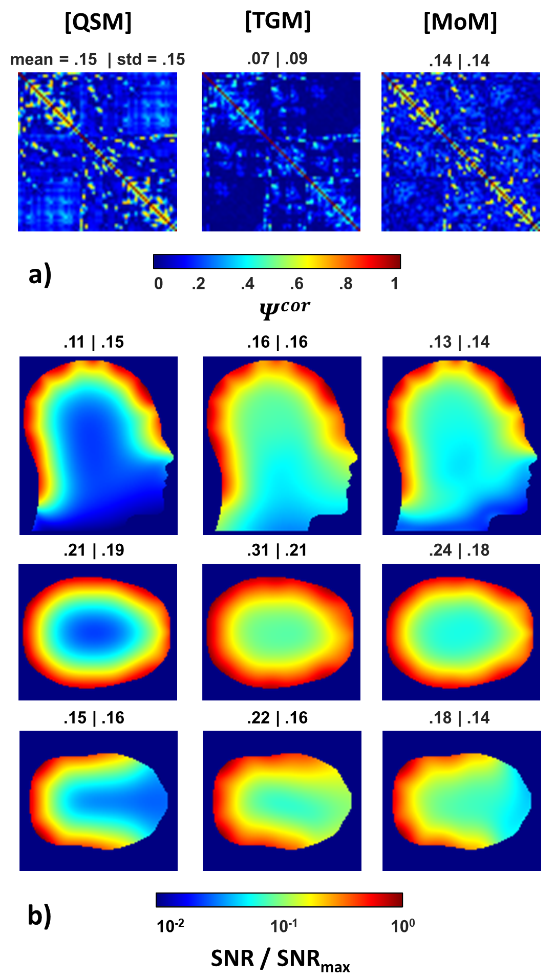
The noise correlation Ψcor (a) and the SNR (b) of the coil array shown in Fig1, calculated using the electric field intensities and the B1- fields obtained with the QSM, the TGM and the MoM. The SNR is shown in all three layers (x=0, z=0, and z=-0.1m).