4192
3D MRI super-resolution using convolutional generative adversarial network with gradient guidance
Wei Xu1, Jing Cheng1, and Dong Liang1
1Shenzhen Institutes of Advanced Technology, Chinese Academy of Sciences, ShenZhen, China
1Shenzhen Institutes of Advanced Technology, Chinese Academy of Sciences, ShenZhen, China
Synopsis
Keywords: Machine Learning/Artificial Intelligence, Brain
The application of MRI has been limited due to the restriction of imaging time and spatial resolution. Super-resolution is an important strategy in clinics to speed up MR imaging. In this work, we propose a novel GAN-based super-resolution method which incorporates gradient features to improve the recovery of local structures of the super-resolution images. Experiments on 3D MR Vessel Wall imaging demonstrate the superior performance of the proposed method.Introduction
Magnetic resonance (MR) imaging is a commonly used medical imaging diagnostic technique in clinical practice. MRI with high spatial resolution can provide rich anatomical information and textural details that facilitate accurate diagnosis of diseases. However, due to hardware conditions and cost constraints, the spatial resolution of clinical MRI is often low, thus limiting its usefulness in disease diagnosis. In this work, we propose a novel method to improve the spatial resolution of 3D MRI while recovering anatomical information and texture details from low-resolution MRI. The experimental results demonstrate the superior performance of the method.Method
We design a convolutional neural network for MRI super-resolution, which takes low-resolution MRI $$$I^{LR}$$$ as input and generates super-resolution images $$$I^{SR}$$$, corresponding to high-resolution images $$$I^{HR}$$$ as ground truth, as shown in Fig 1. We expect super-resolution images to have similar content and structure as high-resolution images. We denote this network as G, which has the parameters $$$\theta_{G}$$$, then we have $$$I^{SR}=G(I^{LR};\theta_{G})$$$. If the loss function $$$L$$$ is used to measure the difference between $$$I^{SR}$$$ and $$$I^{HR}$$$, then our target is to solve the following formulation:$$\theta_{G}^{*}=\mathop{\arg\min}_{\theta_{G}} \mathbb{E}_{I^{SR}}\enspace L(G(I^{LR};\theta_{G}),I^{HR})$$Network Architecture
Our proposed network architecture mainly consists of SR branch and gradient branch, as shown in Fig 1, and the output feature maps of the two branches are finally obtained after a fusion block to generate the super-resolution images. SR branch mainly includes 23 SR blocks and an upsampling block, in which SR block is a convolution block. Here we use the Residual in Residual Dense Block (RRDB) which has been successfully applied in super-resolution field 1, as shown in Fig 2. Simultaneously, gradient branch mainly includes 5 gradient blocks and an upsampling block. The gradient blocks are also RRDB blocks. It is worth noting that the output feature maps of the 5th, 10th, 15th, and 20th SR blocks are input into gradient blocks. M(·) stands for the operation to extract gradient image from original image, the specific calculation formulation for image $$$I(x,y)$$$ is as follows:
$$I_{x}(x)=I(x+1,y)-I(x-1,y),\\I_{y}(x)=I(x,y+1)-I(x,y-1),\\ \nabla I(x)=(I_{x}(x),I_{y}(x)),\\M(I)=||\nabla I||_{2}.$$
Adversarial Training
Generative adversarial networks 2 have been applied in the SR field to recover texture details of super-resolution images 3. We use the aforementioned network as the generator and VGG network 5 as the discriminator, and let them perform adversarial training to improve the realism of super-resolution images. To recover structural details from LR images, adversarial training is introduced in both the original image domain and the gradient image domain 4.
Loss Functions
To reduce the average pixel difference between recovered images $$$I^{SR}$$$ and ground-truths $$$I^{HR}$$$, we introduce pixel loss $$$L_{SR}^{Pix_{I}}$$$:$$L_{SR}^{Pix_{I}} = {\mathbb{E}_{{I^{SR}}}}\enspace ||G({I^{LR}}) - {I^{HR}}||_{1}$$
Perceptual loss can enhance the semantic correlation between recovered images and ground-truths 6, which is defined as follows:$$L_{SR}^{Per} = {\mathbb{E}_{{I^{SR}}}}\enspace||{\phi _i}(G({I^{LR}})) - {\phi _i}({I^{HR}})|{|_1}$$where $$$\phi _i$$$ is a pretrained VGG network 5.
Since we employ adversarial training, there are adversarial losses for generator$$$L_{SR}^{Ad{v_I}}$$$ and discriminator $$$L_{SR}^{Di{s_I}}$$$: $$L_{SR}^{Ad{v_I}} = - {\mathbb{E}_{{I^{SR}}}}[\log {D_I}(G({I^{LR}}))]\\$$ $$L_{SR}^{Di{s_I}} = - {E_{{I^{SR}}}}[\log (1 - {D_I}({I^{SR}}))] - {\mathbb{E}_{{I^{HR}}}}[\log {D_I}({I^{HR}})]$$
Similarly, in the gradient image domain, gradient pixel loss $$$L_{SR}^{Pi{x_{GI}}}$$$ , gradient adversarial losses for generator $$$L_{SR}^{Ad{v_{GI}}}$$$ and discriminator $$$L_{SR}^{Di{s_{GI}}}$$$ and branch pixel loss $$$L_{GB}^{Pi{x_{GI}}}$$$ are introduced:
$$L_{SR}^{Pi{x_{GI}}} = {\mathbb{E}_{{I^{SR}}}}||M(G({I^{LR}})) - M({I^{HR}})|{|_1}$$
$$L_{SR}^{Ad{v_{GI}}} = - {\mathbb{E}_{{I^{SR}}}}[\log {D_{GI}}(M(G({I^{LR}})))]$$
$$L_{SR}^{Di{s_{GI}}} = - {\mathbb{E}_{{I^{SR}}}}[\log (1 - {D_{GI}}(M({I^{SR}})))] - {\mathbb{E}_{{I^{HR}}}}[\log {D_{GI}}(M({I^{HR}}))]$$
$$L_{GB}^{Pi{x_{GI}}} = {\mathbb{E}_{{I^{SR}}}}\enspace ||GB({I^{LR}}) - M({I^{HR}})|{|_1}$$
where $$$GB({I^{LR}})$$$ is the Reconstructed Grad in Fig 1.
Therefore, the overall loss function of the generator is as follows:$$L^{G}=L_{SR}^{G}+L_{GI}^{G}= L_{SR}^{Per} + \beta _{SR}^IL_{SR}^{Pi{x_I}} + \gamma _{SR}^IL_{SR}^{Ad{v_I}} + \beta _{SR}^{GI}L_{SR}^{Pi{x_{GI}}} + \gamma _{SR}^{GI}L_{SR}^{Ad{v_{GI}}} + \beta _{GB}^{GI}L_{GB}^{Pi{x_{GI}}}$$
where these constants $$$\beta$$$ and $$$\gamma$$$ are used to make trade-offs for these losses.
Experiments
The details of the experiments are described below. First, regarding the experimental data, fully sampled multi-channel brain vessel wall images of four volunteers were collected out of which data from three subjects were used for training, while the data from the fourth subject were used for testing. Each subject has dimensions in rows×columns×slices×coils as 336×280×368×20. We make these data into a convenient dataset for network training and testing, as shown in the Fig 3. Second, the details of the experimental implementation are as follows. Due to the setting of the data dimensions, scaling factor of our network is 2. We set the learning rates to 1 ×10⁻⁴ for both generator and discriminator, and ADAM optimizor with $$$\beta_1= 0.9$$$,$$$\beta_2= 0.999$$$ is used for optimization. As for the trade-off parame-ters of losses, we set $$$ \beta _{SR}^I=\beta _{SR}^{GI}=0.01$$$, $$$\gamma _{SR}^I=\gamma _{SR}^{GI}=0.005$$$,$$$\beta _{GB}^{GI}=0.5$$$. Such a setting can enhance the perceptual quality of SR images.Results
We compare the output SR images of our model in the axial and sagittal surfaces with LR images, zero-filling images, and the results of SRGAN 3. As can be seen from Fig 4 and 5, our model recovers anatomical information and texture details better than LR and other methods.Conclusion
In this work, we propose a novel method for 3D MRI super-resolution. By applying our proposed convolutional generative adversarial network model, the resolution of the original low-resolution MRI of the vascular wall of the brain is improved, while anatomical information and textural details are well recovered. Our proposed model can be well applied to improve the resolution of brain vessel wall MRI in the future.Acknowledgements
No acknowledgement found.References
- Xintao Wang, Ke Yu, Shixiang Wu, Jinjin Gu, Yihao Liu,Chao Dong, Yu Qiao, and Chen Change Loy. Esrgan: Enhanced super-resolution generative adversarial networks. In ECCV, pages 63–79.
- Goodfellow, Ian; Pouget-Abadie, Jean; Mirza, Mehdi; Xu, Bing; Warde-Farley, David; Ozair, Sherjil; Courville, Aaron; Bengio, Yoshua (2014). Generative Adversarial Nets. Proceedings of the International Conference on Neural Information Processing Systems (NIPS 2014). pp. 2672–2680.
- Christian Ledig, Lucas Theis, Ferenc Husz ́ar, Jose Caballero, Andrew Cunningham, Alejandro Acosta, Andrew Aitken, Alykhan Tejani, Johannes Totz, Zehan Wang, et al. Photo-realistic single image super-resolution using a generative adversarial network. In CVPR, pages 4681–4690, 2017.
- Ma Cheng, Rao Yongming, Cheng Yean, Chen Ce, Lu Jiwen, Zhou Jie, "Structure-Preserving Super Resolution With Gradient Guidance," 2020 IEEE/CVF Conference on Computer Vision and Pattern Recognition (CVPR), 2020, pp. 7766-7775.
- Karen Simonyan and Andrew Zisserman. Very deep convolutional networks for large-scale image recognition. arXiv preprint arXiv:1409.1556, 2014.
- Justin Johnson, Alexandre Alahi, and Li Fei-Fei. Perceptual losses for real-time style transfer and super-resolution. In ECCV, pages 694–711. Springer, 2016.
Figures
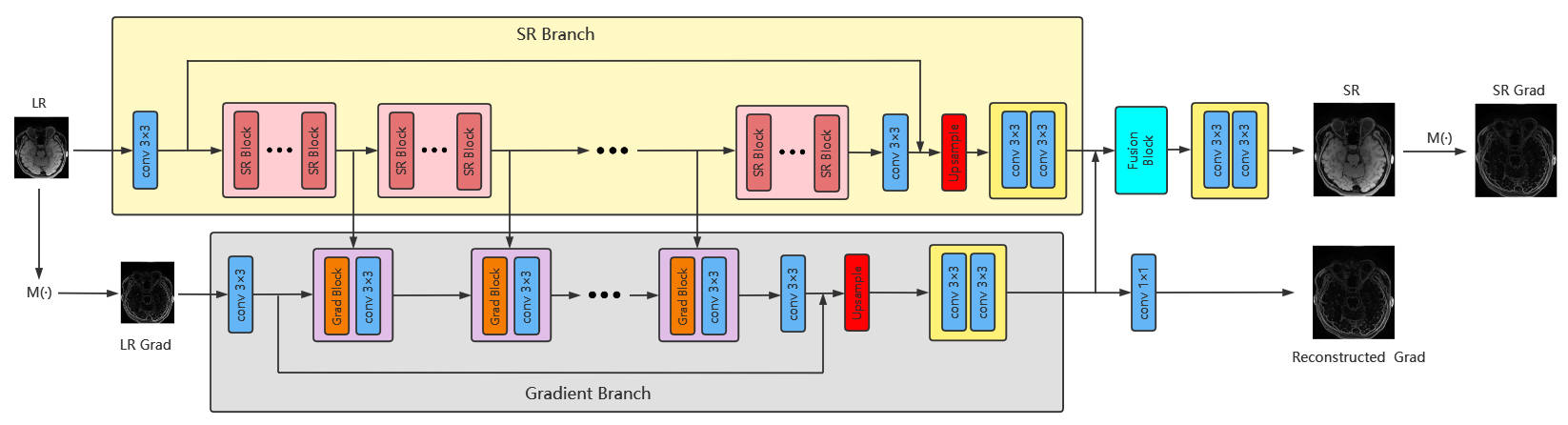
Fig1. Our proposed network architecture. The architecture mainly consists of SR branch and gradient branch. The SR branch learns texture detail features to generate SR images. The gradient branch learns structural features and fuses multi-level representations from SR branch to aid in SR image generation.
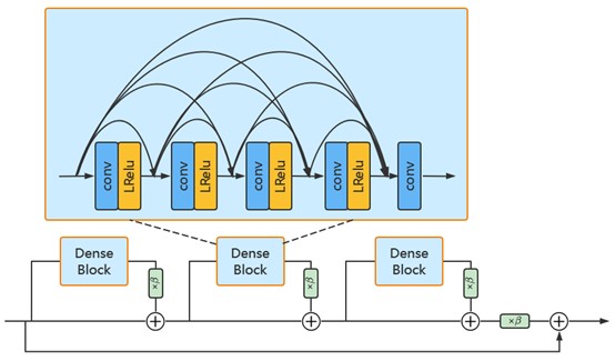
Fig2. The Residual in Residual Dense Block (RRDB). It includes three Dense Blocks, as well as a global skip connection and three local skip connections. Each Dense Block has five convolutional layers, the first four of which connect LeakyReLU as activation. Dense connections are introduced between these five convolutional layers simultaneously.
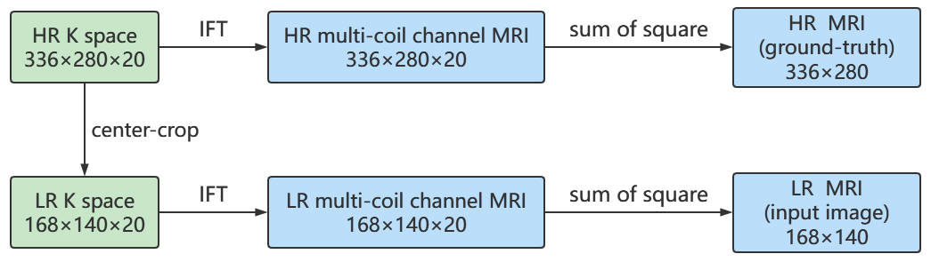
Fig3. Flow chart of data pre-processing. We have high-resolution (HR) K space of dimensions in rows×columns×coils as 336×280×20. Then we performed inverse Fourier transform (IFT) to obtain HR multi-coil channel MRI. We finally performed coil channel fusion by sum of square to get single channel HR MRI and use it as ground-truth. Meanwhile, to obtain low-resolution (LR) MRI, we first center crop the HR K space to reduce the resolution to half of the original. The subsequent process is similar to the HR case.
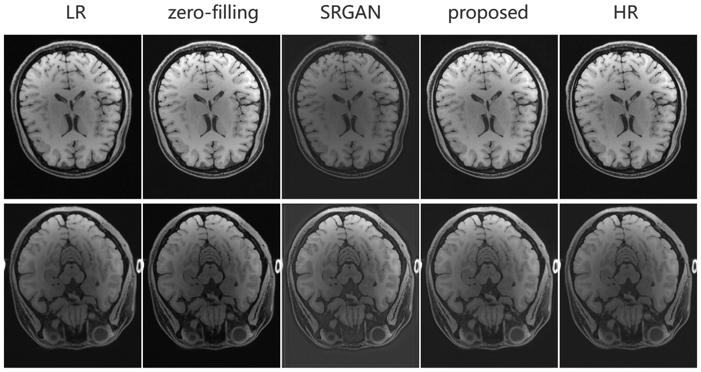
Fig4. Super-resolution results of axial
view. We can see that the edges of LR are blurred, the texture details of LR and zero-fill images are not rich
enough, the results of SRGAN have stripe artifacts and the results of our
proposed method behave most similarly to HR.
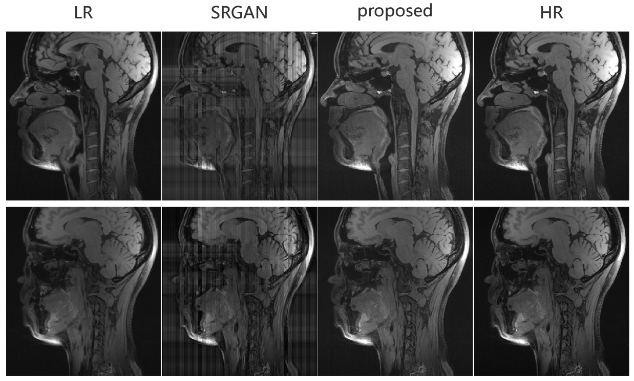
Fig5. Super-resolution results of
sagittal view. We can see that the edges of LR are blurred and the texture detail is not rich enough, the results of SRGAN have stripe
artifacts and the results of our proposed method also show the most similarity
to HR.
DOI: https://doi.org/10.58530/2023/4192