4186
Dynamic Geometric Distortion Correction for Quantitative Susceptibility Mapping Using a Multi-Echo 2D-EPI Sequence
Oliver C. Kiersnowski1, Patrick Fuchs1, Stephen J. Wastling2,3, John S. Thornton2,3, and Karin Shmueli1
1Department of Medical Physics and Biomedical Engineering, University College London, London, United Kingdom, 2Neuroradiological Academic Unit, UCL Queen Square Institute of Neurology, University College London, London, United Kingdom, 3Lysholm Department of Neuroradiology, National Hospital for Neurology and Neurosurgery, London, United Kingdom
1Department of Medical Physics and Biomedical Engineering, University College London, London, United Kingdom, 2Neuroradiological Academic Unit, UCL Queen Square Institute of Neurology, University College London, London, United Kingdom, 3Lysholm Department of Neuroradiology, National Hospital for Neurology and Neurosurgery, London, United Kingdom
Synopsis
Keywords: Susceptibility, Quantitative Susceptibility mapping
Echo planar imaging (EPI) suffers from geometric distortions, which can be corrected using reference acquisitions for single-echo EPI, or using field maps calculated from the multiple echoes in multi-echo EPI. The effect of distortion on EPI quantitative susceptibility mapping (QSM) has not been investigated. We compared static and dynamic geometric distortion correction for magnitude images and QSM using multi-echo 2D-EPI acquisitions with and without changes in head position. Multi-echo EPI corrected distortion in both magnitude and QSM images without the need for reference scans. Correcting the local field map in the QSM pipeline was optimal to reduce temporal variance.Introduction
Echo planar imaging (EPI) has been used for structural1 and functional2–4 quantitative susceptibility mapping (QSM)5, but suffers from geometric distortion. Single-echo EPI distortion correction can be applied using a static field map obtained from a reference scan6, or dynamically using field maps estimated for each timepoint7,8. Multi-echo (ME) EPI has the advantage that dynamic field maps can be calculated by fitting the phase over multiple echo times9, obviating any reference scans. It is unknown where in the QSM pipeline to apply distortion correction optimally. Therefore, we applied static and dynamic distortion correction at three points in the QSM pipeline to investigate the effect of distortion on the accuracy of susceptibility ($$$\chi$$$) values and to determine the optimal point to apply correction.Methods
AcquisitionA healthy volunteer was imaged on a 3T Siemens Prisma MR system using a 64-channel head coil. A reference 3D-GRE scan was acquired at 1mm isotropic resolution with echo times: TE1/ΔTE/TE4=4.92/4.92/19.68 ms; TR=30 ms; GRAPPA=3; 6/8 phase partial Fourier; FOV=256x256x192 mm; Ttot=7min 25s.
A single-shot 2D-EPI10 scan was used twice to acquire 70 timepoints at 1.5 mm isotropic resolution with TE=12.8, 33.71, 54.62 ms; TR=3346 ms; GRAPPA=4; multiband factor 3; Ttot=5min11s. At three times during the second run, the volunteer changed their head position, causing dynamic geometric distortions and allowing static and dynamic correction methods to be compared.
A standard structural reference image was acquired using a T1-weighted MPRAGE sequence at 1mm isotropic resolution.
Distortion correction
Using FSL FUGUE11, three methods were applied to correct the BOLD-optimised combined12 magnitude images, and QSMs at three points in the QSM pipeline: (i) the total field map (TFM), (ii) local field map (LFM) and (iii) the final susceptibility map (FSM), using the following field maps:
- sGRE: a static, reference field map calculated from the 3D-GRE acquisition was applied to each EPI timepoint.
- sEPI: a static field map calculated from the first EPI timepoint was applied to each subsequent timepoint.
- dEPI: dynamic field maps were calculated and applied at each EPI timepoint.
Field map calculation
The static field map for sGRE was calculated using a non-linear fit13 of the GRE complex data over all TEs with residual phase wraps unwrapped using SEGUE14. This was registered to each EPI volume using an affine transformation obtained by rigidly registering the first echo magnitude images of the GRE and EPI with NifyReg15, followed by ‘forward warping’ the GRE map into the EPI space by applying the inverse of the field map’s distortion correction to itself8.
Field maps for sEPI and dEPI were calculated at each EPI volume using a non-linear fit13 of the field-corrected16 EPI complex data over all TEs and SEGUE14 phase unwrapping. The first volume EPI field map was used for sEPI.
Brain masks for all field maps were obtained using FSL BET17 on the first-echo magnitude images, from their respective GRE/EPI acquisition. To improve distortion correction at the edges of the brain, regions outside the brain were set to NaNs and field maps were extrapolated well beyond the brain edges using MATLAB function smoothn.m18 with smoothing parameter=2, as in Dymerska et al.8.
QSM pipeline
GRE and EPI $$$\chi$$$ maps were reconstructed via Laplacian unwrapping19 of the fitted field maps used in the field map calculations, followed by PDF20 background field removal (plus 2D/3D V-SHARP for EPI21,22) and non-linear total variation $$$\chi$$$ calculation23,24 (α=2×10⁻⁵ and α=1×10⁻⁴ for GRE and EPI, respectively). Average susceptibility maps were calculated by averaging maps that were initially co-registered to the first volume across all (non-motion corrupted) timepoints.
Statistical Analysis
The temporal standard deviation ($$$\sigma$$$/$$$\sigma_\chi$$$) between uncorrected and corrected magnitude images / susceptibility maps were compared visually and using Kruskal-Wallis tests to identify differences in the medians of brain $$$\sigma$$$ distributions by statistically comparing the mean ranks of the distributions. Mean $$$\chi$$$ values within five ROIs (segmented using MRICloud25,26) were compared for all correction methods.
Results and Discussion
Head position changes led to different distortions (Figure 1, top row), which were corrected well by static field maps obtained in the same position (Figure 1, left) but were poorly corrected at a different position (Figure 1, right). Dynamic EPI field maps (dEPI) accurately corrected distortion in all positions (Figure 1, bottom row) and reduced $$$\sigma$$$ (Figure 2a). $$$\sigma$$$ was reduced the most by sGRE when the subject’s head did not change position but by dEPI when the head did change position (Figure 2b). Head movement led to large regional $$$\chi$$$ shifts that were not removed by distortion correction (Figure 3). However, all correction methods reduced $$$\sigma_\chi$$$ (Figure 4) compared to the uncorrected $$$\chi$$$ map. dEPI reduced $$$\sigma_\chi$$$ inside the brain more than sGRE and sEPI (Figure 4, yellow arrows). Distortion correction of the LFM reduced $$$\sigma_\chi$$$ the most for all correction methods, while correcting the FSM reduced $$$\sigma_\chi$$$ the least (Figure 5a). Corrected averaged susceptibility maps display small differences compared to uncorrected (Figure 5b).Conclusions
Dynamic distortion correction from ME-EPI reduced distortion in the magnitude and $$$\chi$$$ maps without need for additional reference scans. Distortion correction applied to the local field map reduced temporal variability in $$$\chi$$$ the most, which is relevant for functional QSM applications.Acknowledgements
Oliver Kiersnowski’s work was supported by the EPSRC-funded UCL Centre for Doctoral Training in Intelligent, Integrated Imaging in Healthcare (i4health) (EP/S021930/1). John Thornton received support from the National Institute for Health Research University College London Hospital Biomedical Research Centre. Karin Shmueli and Patrick Fuchs were supported by European Research Council Consolidator Grant DiSCo MRI SFN 770939.References
- Sun H, Wilman AH. Quantitative susceptibility mapping using single-shot echo-planar imaging. Magn Reson Med. 2015;73(5):1932-1938. doi:10.1002/mrm.25316
- Balla DZ, Sanchez-Panchuelo RM, Wharton SJ, et al. Functional quantitative susceptibility mapping (fQSM). Neuroimage. 2014;100:112-124. doi:10.1016/j.neuroimage.2014.06.011
- Sun H, Seres P, Wilman AH. Structural and functional quantitative susceptibility mapping from standard fMRI studies. NMR Biomed. 2017;30(4). doi:10.1002/nbm.3619
- Özbay PS, Warnock G, Rossi C, et al. Probing neuronal activation by functional quantitative susceptibility mapping under a visual paradigm: A group level comparison with BOLD fMRI and PET. Neuroimage. 2016;137:52-60. doi:10.1016/j.neuroimage.2016.05.013
- Shmueli K. Quantitative Susceptibility Mapping. In: Quantitative Magnetic Resonance Imaging. 1st ed. Elsevier; 2020.
- Jezzard P, Balaban RS. Correction for geometric distortion in echo planar images from B0 field variations. Magn Reson Med. 1995;34(1):65-73. doi:10.1002/mrm.1910340111
- Dymerska B, Poser BA, Bogner W, et al. Correcting dynamic distortions in 7T echo planar imaging using a jittered echo time sequence. Magn Reson Med. 2016;76(5):1388-1399. doi:10.1002/mrm.26018
- Dymerska B, Poser BA, Barth M, Trattnig S, Robinson SD. A method for the dynamic correction of B0-related distortions in single-echo EPI at 7 T. Neuroimage. 2018;168:321-331. doi:10.1016/j.neuroimage.2016.07.009
- Hutton C, Bork A, Josephs O, Deichmann R, Ashburner J, Turner R. Image distortion correction in fMRI: A quantitative evaluation. Neuroimage. 2002;16(1):217-240. doi:10.1006/nimg.2001.1054
- Center for Magnetic Resonance Research Department of Radiology. Multi-Band Accelerated EPI Pulse Sequences. https://www.cmrr.umn.edu/multiband/
- Jenkinson M, Beckmann CF, Behrens TEJ, Woolrich MW, Smith SM. FSL. Neuroimage. 2012;62(2):782-790. doi:10.1016/j.neuroimage.2011.09.015
- Poser BA, Norris DG. Investigating the benefits of multi-echo EPI for fMRI at 7 T. Neuroimage. 2009;45(4):1162-1172. doi:10.1016/j.neuroimage.2009.01.007
- Liu T, Wisnieff C, Lou M, Chen W, Spincemaille P, Wang Y. Nonlinear formulation of the magnetic field to source relationship for robust quantitative susceptibility mapping. Magn Reson Med. 2013;69(2):467-476. doi:10.1002/mrm.24272
- Karsa A, Shmueli K. SEGUE: A Speedy rEgion-Growing Algorithm for Unwrapping Estimated Phase. IEEE Trans Med Imaging. 2019;38(6):1347-1357. doi:10.1109/TMI.2018.2884093
- Modat M, Cash DM, Daga P, Winston GP, Duncan JS, Ourselin S. Global image registration using a symmetric block-matching approach. Journal of Medical Imaging. 2014;1(2):024003. doi:10.1117/1.jmi.1.2.024003
- MEDI Toolbox. http://pre.weill.cornell.edu/mri/pages/qsm.html
- Smith SM. Fast robust automated brain extraction. Hum Brain Mapp. 2002;17(3):143-155. doi:10.1002/hbm.10062
- Garcia D. Robust smoothing of gridded data in one and higher dimensions with missing values. Comput Stat Data Anal. 2010;54(4):1167-1178. doi:10.1016/j.csda.2009.09.020
- Schofield MA, Zhu Y. Fast phase unwrapping algorithm for interferometric applications. Opt Lett. Published online 2003. doi:10.1364/ol.28.001194
- Liu T, Khalidov I, de Rochefort L, et al. A novel background field removal method for MRI using projection onto dipole fields (PDF). NMR Biomed. 2011;24(9):1129-1136. doi:10.1002/nbm.1670
- Wei H, Zhang Y, Gibbs E, Chen NK, Wang N, Liu C. Joint 2D and 3D phase processing for quantitative susceptibility mapping: application to 2D echo-planar imaging. NMR Biomed. 2017;30(4). doi:10.1002/nbm.3501
- Li W, Wu B, Liu C. Quantitative susceptibility mapping of human brain reflects spatial variation in tissue composition. Neuroimage. 2011;55:1645-1656. doi:10.1016/j.neuroimage.2010.11.088
- Milovic C, Bilgic B, Zhao B, Acosta-Cabronero J, Tejos C. Fast nonlinear susceptibility inversion with variational regularization. Magn Reson Med. 2018;80(2):814-821. doi:10.1002/mrm.27073
- FANSI Toolbox. https://gitlab.com/cmilovic/FANSI-toolbox
- Li X, Chen L, Kutten K, et al. Multi-atlas tool for automated segmentation of brain gray matter nuclei and quantification of their magnetic susceptibility. Neuroimage. 2019;191:337-349. doi:10.1016/j.neuroimage.2019.02.016
- Mori S, Wu D, Ceritoglu C, et al. MRICloud: Delivering high-throughput MRI neuroinformatics as cloud-based software as a service. Comput Sci Eng. 2016;18(5):21-35. doi:10.1109/MCSE.2016.93
Figures
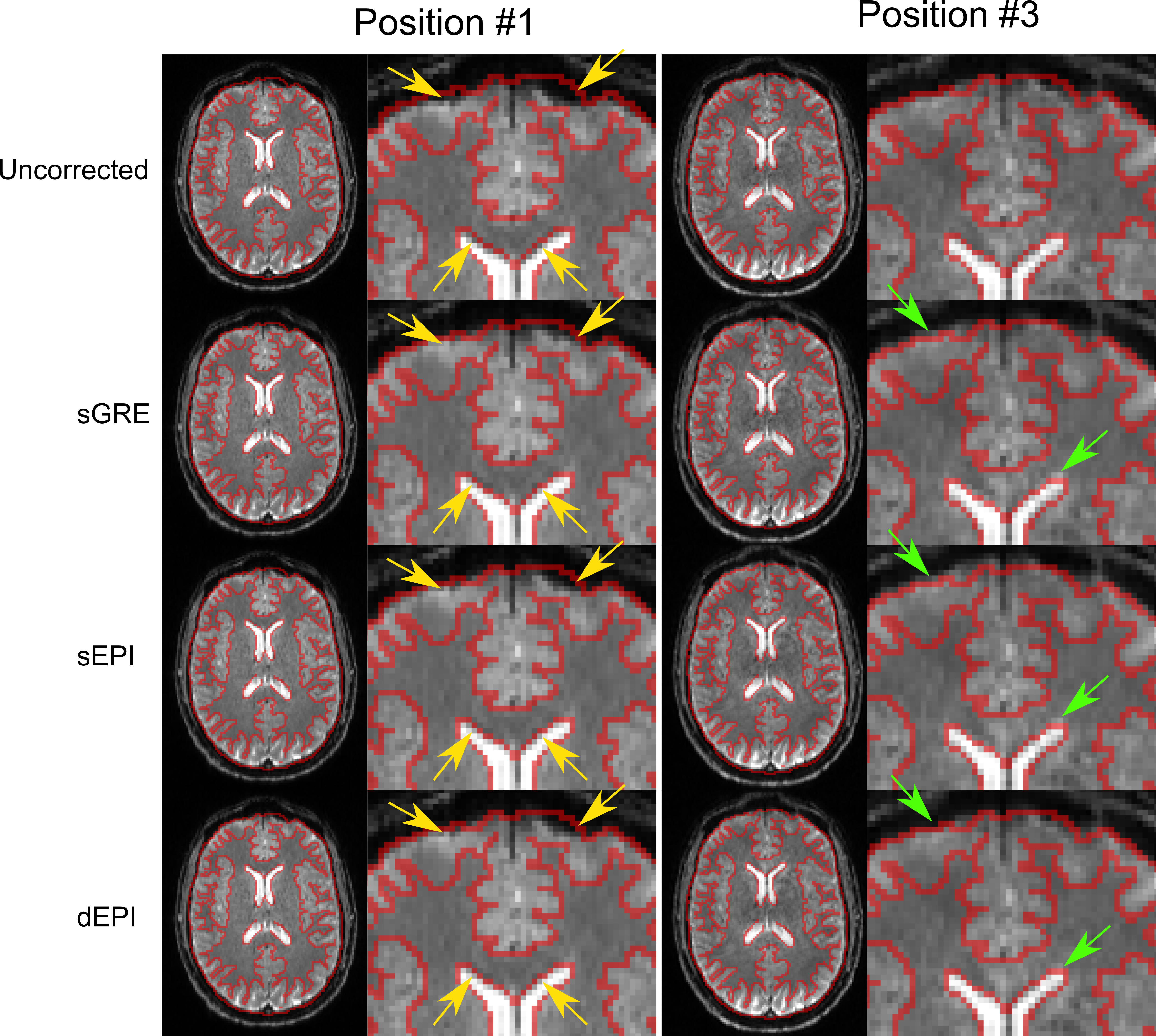
Figure 1: EPI magnitude
images at position #1 (left) and #3 (right) with red outlines drawn on the T1
weighted structural image (not shown). Uncorrected images at different
head positions show different distortions (top). The sGRE, sEPI and dEPI corrected images in position #1 are similar in the brain (yellow
arrows) with sGRE outperforming EPI at the brain edges. In position #3, sGRE and sEPI inaccurately over-correct distortions in the brain
and at the edges compared to dEPI (green arrows).
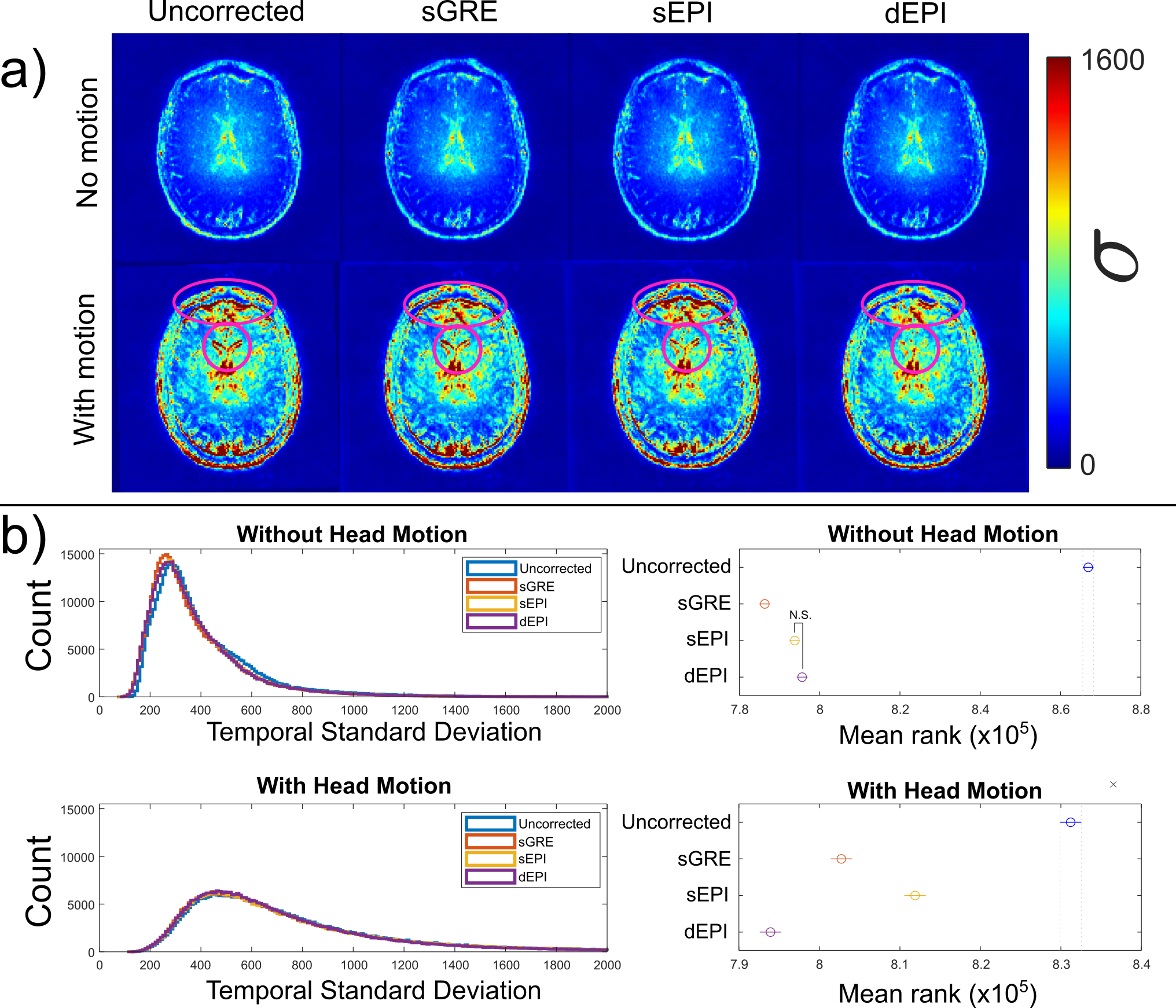
Figure 2: (a) Temporal
standard deviation (σ) maps
of the EPI magnitude images for EPI runs with and without changes in head
position. Unlike sGRE and sEPI, dEPI
reduced high σ, due to distortions
from position changes, at the front and centre of the brain (pink ellipses) but
sEPI and sGRE did not. (b) Histograms of σ (left), with their mean ranks (right)
reflecting the distributions’ medians. Kruskal-Wallis tests showed that dEPI reduced σ significantly more than sGRE and sEPI when head
position changed (N.S. = not significant).
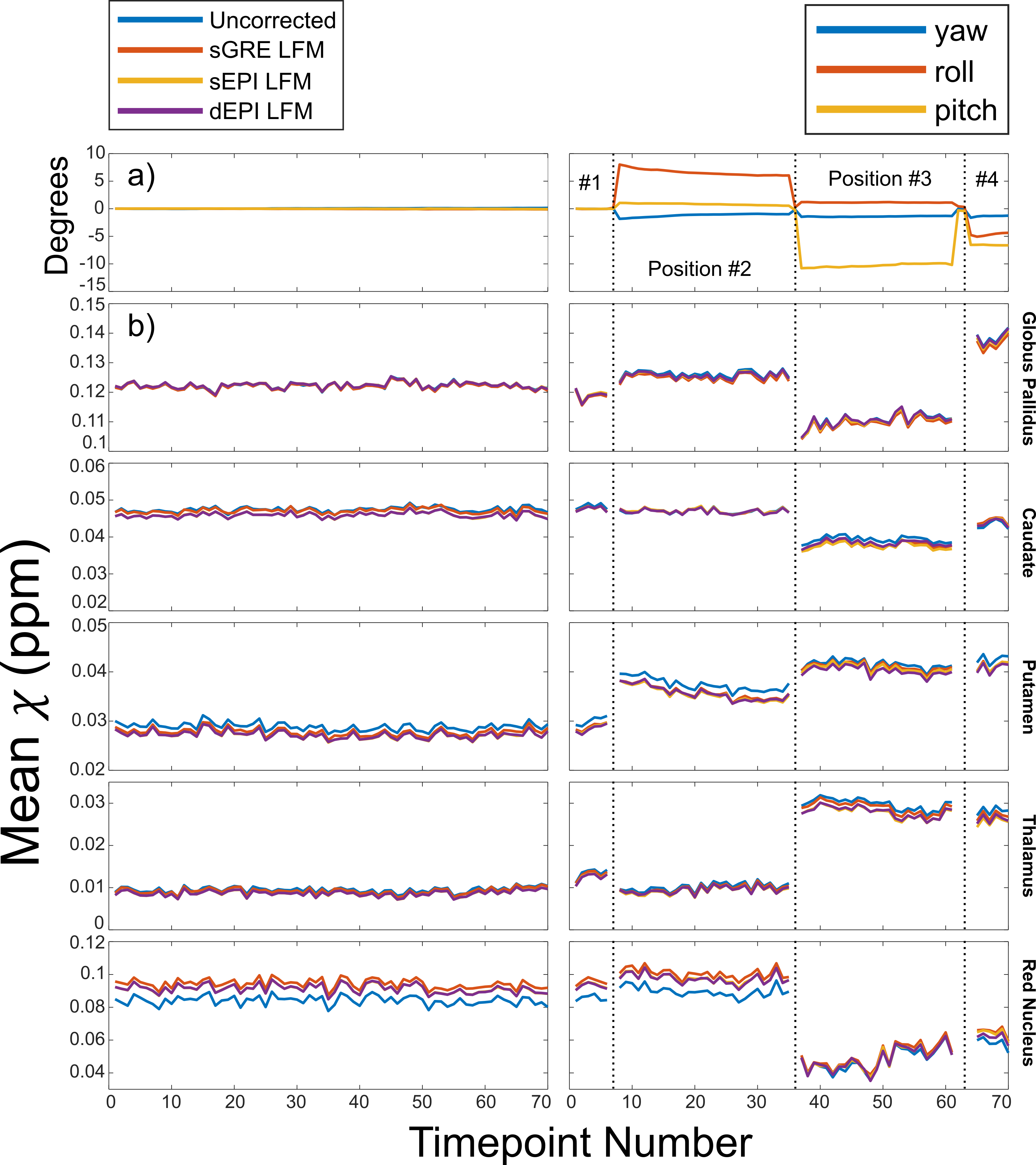
Figure 3: Mean
susceptibilities for the scan without (left) and with (right) head position
changes. (a) Angles of rotation for the different head positions. (b) Temporal χ in five regions of interest. Dotted lines show
position changes. These caused much larger changes in χ than those caused by geometric distortion.
Therefore, distortion correction did not improve the accuracy of mean regional χ when the head changed position. Motion
corrupted volumes were removed.
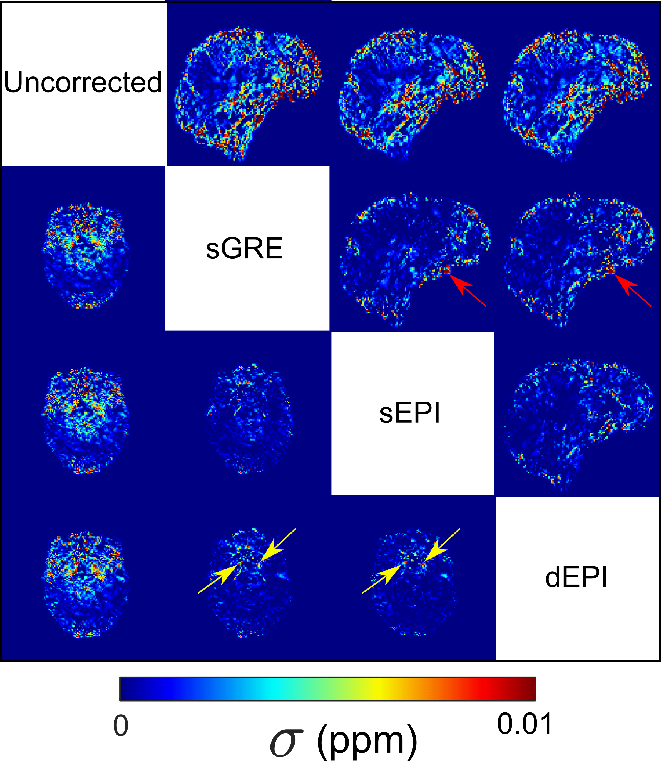
Figure 4: Axial and sagittal
slices of σχ difference images (showing
positive differences only) between uncorrected and distortion corrected χ maps. All methods showed some σχ reductions
in areas prone to distortion (red: σχ was higher in uncorrected than corrected maps).
Red arrows indicate σχ differences between sGRE and
EPI-based correction due to differences in distortion correction at the brain
edges. Yellow arrows indicate small improvements of dEPI over sEPI and sGRE
methods, as seen for magnitude images (Figure 1a).
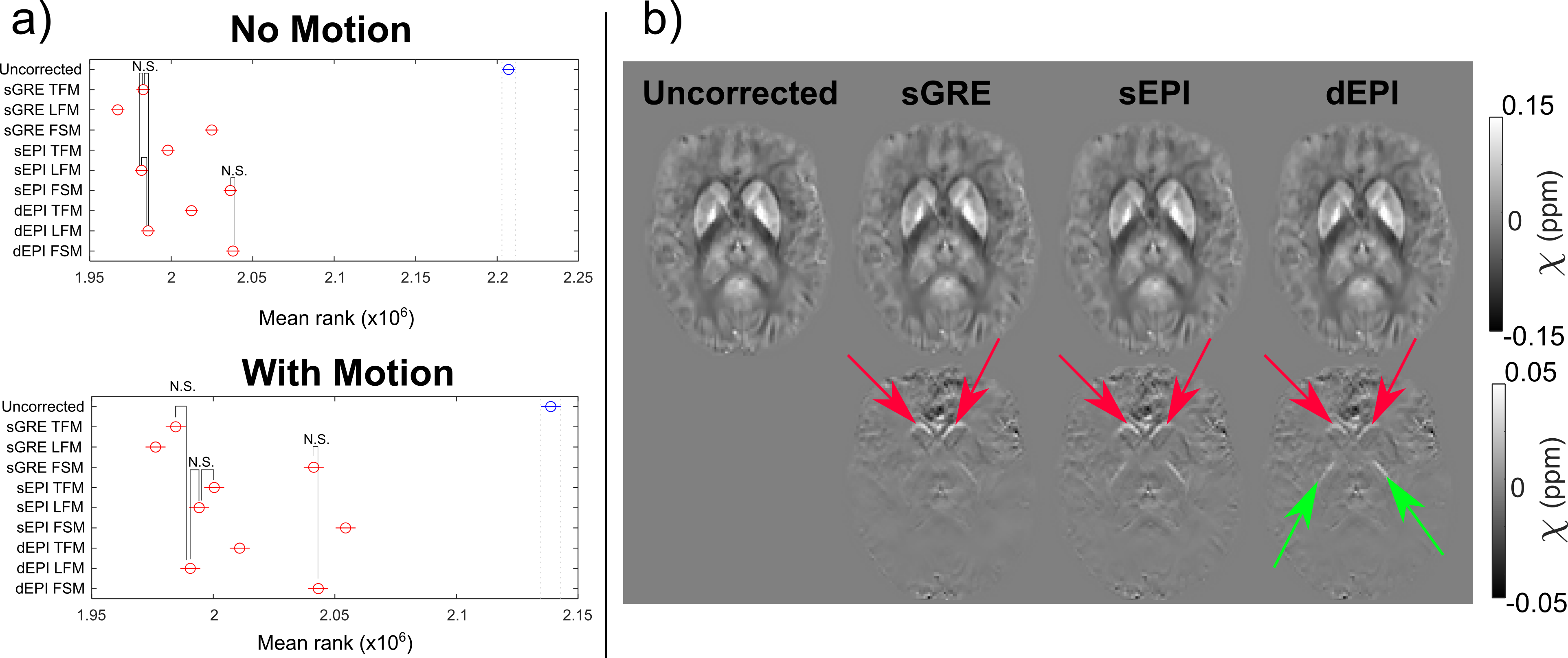
Figure 5: (a) Mean σχ distribution ranks, reflecting the median σχ, for
scans with and without head position changes show that applying all distortion correction methods
to the local field map (LFM) reduced the σχ most but correcting the final χ map (FSM) reduced σχ the least. (b) The LFM-corrected average χ maps (top) and difference maps (bottom) for the
acquisition with head position changes show that correction shifts the caudate
nucleus (red arrows) and globus pallidus (green arrows).
DOI: https://doi.org/10.58530/2023/4186