4177
Including mesoscopic frequency shifts from fibrous structure of white matter improves accuracy of QSM1Center for functionally integrative neuroscience, department of clinical medicine, Aarhus University, Aarhus, Denmark, 2Division of Medical Physics, Department of Radiology, University Medical Center Freiburg, Freiburg, Germany, 3Champalimaud Research, Champalimaud Centre for the Unknown, Lisbon, Portugal, 4Department of Phsysics and Astronomy, Aarhus University, Aarhus, Denmark
Synopsis
Keywords: Microstructure, Quantitative Susceptibility mapping
Quantitative Susceptibility Mapping (QSM) is a highly utilized MRI modality for mapping tissue susceptibility. However, a limitation of QSM is disregarding mesoscopic field effects associated with WM microstructure and anisotropic susceptibility. Here we present a minimal extension of QSM by including frequency shifts due to the fibrous WM microstructure, while still neglecting susceptibility anisotropy and WM spherical inclusions modelling iron complexes. We find that this step already improves the accuracy of QSM as it is shown by comparison with conventional QSM using a digital phantom that includes microstructural frequency shifts from multiple sources.Introduction
Quantitative susceptibility mapping (QSM) is a promising method for imaging changes in tissue iron, calcium and myelin1-4. However, one of the shortcomings of QSM is neglecting mesoscopic fields associated with microstructure and anisotropic susceptibility5-7. These assumptions are challenged especially in white matter (WM), where field perturbations from myelinated axons depend on the orientation to the external field $$$\mathbf{B}_0$$$ due to its magnetic and structural anisotropy5-7. We recently presented an analytical solution for the frequency shift in WM (Figure 1A_D) including both myelinated axons and spherical inclusions8. Unfortunately, estimating all its parameters require active rotation of the sample with respect to $$$\mathbf{B}_0$$$, which may not be practical in most scanners.Here we investigate the parameter accuracy of QSM in a digital phantom compared to a constrained version of our model which (A) includes mesoscopic frequency shifts due to fibrous WM microstructure, (B) neglects susceptibility anisotropy of myelin and (C) neglects spherical inclusions in WM. The model represents a minimal framework for including mesoscopic effects when imaging at multiple orientations is not an option. Last, we investigate the effect of including (A)-(C) in QSM when estimating susceptibility of real MRI data.
Methods
Theory: The main assumption in QSM9 is that the measured frequency shift $$$\overline\Omega_{\mathrm{MRI}}$$$ can be described by induced shifts only from other voxels, i.e. on the macroscale: $$\overline\Omega_{\mathrm{MRI}}(\mathbf{R})=\sum_{\mathbf{R}^{'}}\Upsilon(\mathbf{R}^{'}-\mathbf{R})\overline\chi(\mathbf{R}^{'})\quad(1)$$Here $$$\Upsilon(\mathbf{R})$$$ defines the dipole field assuming the external field is along $$${\hat{z}}$$$ and $$$\overline\chi(\mathbf{R})$$$ the bulk magnetic susceptibility of voxel $$$\mathbf{R}$$$. We denote the model MACRO.
Our proposed model includes mesoscopic frequency shift in WM, described by a mask $$$\tilde{\mathrm{M}}_{\mathrm{WM}}$$$, which we denote MESO+MACRO. The forward model thus becomes $$\overline\Omega_{\mathrm{MRI}}(\mathbf{R})=-\frac{1}{3}\overline\chi(\mathbf{R})\tilde{\mathrm{M}}_{\mathrm{WM}}(\mathbf{R})\sum_{m}p_{2m}(\mathbf{R})\mathrm{Y}_2^m(\hat{z})+\sum_{\mathbf{R}^{'}}\Upsilon(\mathbf{R}^{'}-\mathbf{R})\overline\chi(\mathbf{R}^{'})\quad(2)$$
Here $$$p_{2m}$$$ is the Laplace expansion coefficients of the fiber orientation distribution (fODF), $$$\mathrm{Y}_2^m$$$ spherical harmonics .
Phantom Simulation: We tested the accuracy in susceptibility fitting of the two models on a digital phantom with piece-wise constant susceptibility. It is based on dMRI measurements of an ex-vivo mouse brain at 16.4T with 100μm isotropic resolution. Data was denoised using tensor-MPPCA10 and subsequently Gibbs-unrung11. From DKI12 fitting (b=0,3,5ms/µm2, 30 dir.) we extracted FA and MD. We segmented the brain into gray and WM by creating a binary mask $$$\tilde{\mathrm{M}}_{\mathrm{WM}}$$$ from high FA regions (figure 1E). $$$p_{2m}$$$ was estimated using FBI13 (b=10ms/µm2, 75 dir.). From these, we synthesized 4 susceptibility parameters:
$$\overline\chi_\perp=-5\cdot\mathrm{FA}\cdot\tilde{\mathrm{M}}_{\mathrm{WM}}\\{\Delta}\overline\chi=1\cdot\mathrm{FA}\cdot\tilde{\mathrm{M}}_{\mathrm{WM}}\\{\overline\chi}_{GM}^S\propto\mathrm{MD}\cdot(1-\tilde{\mathrm{M}}_{\mathrm{WM}})\\{\overline\chi}_{WM}^S\propto\mathrm{MD}\cdot\tilde{\mathrm{M}}_{\mathrm{WM}}$$
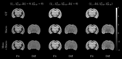
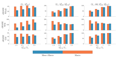
Here $$$\Delta\overline\chi=\chi_\parallel-\chi_\perp$$$. The proportionality indicates that we consider various ratios of spherical susceptibility compared to WM. Three phantoms of increasing complexity were investigated with different combinations of susceptibility and denoted GT in Figure 2 while the titles indicate the added sources. We generated the corresponding frequency shift for each phantom and added noise corresponding to an SNR of 50. We then estimated the susceptibility using either Eq. (1) or (2). For this we used the LSMR14 algorithm.
Ex-vivo susceptibility fitting: We acquired multi-echo gradient data (t=1.75,3.5,..,35 ms) of the mouse brain at 100µm isotropic resolution and similar processing to dMRI. Phase unwrapping was done using SEGUE15 and LBV16 was utilized for background field removal. The estimated Larmor frequency $$$\overline\Omega_{\mathrm{MRI}}$$$ was used to fit susceptibility to either Eq. (1) or (2), again using LSMR.
Results
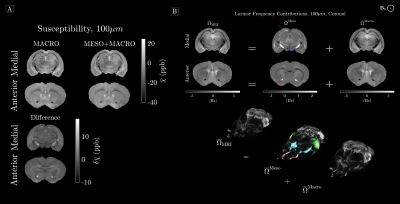
Phantom Simulation: Figure 2 shows the resulting susceptibility fits for all three phantoms along with the difference to ground truth. It is clear to see from the residuals that WM is less biased. Figure 3 shows the normalized RMSE for all three phantoms, and here we find that our constrained model has the lowest RMSE, as long as $$$\overline\chi_\perp\geq\overline\chi_{WM}^S$$$.Ex-vivo fitting: Figure 4 shows the resulting susceptibility fits using either Eq. (1) or (2). Here we find up to 56% change in susceptibility in highly anisotropic WM, when using our model. Figure 4 shows the resulting mesoscopic $$$\overline\Omega^{\mathrm{Meso}}$$$ and macroscopic $$$\overline\Omega^{\mathrm{Macro}}$$$ frequency shift, respectively. Here we find that $$$\overline\Omega^{\mathrm{Meso}}$$$ has a magnitude up to 70% of the total frequency shift in highly anisotropic WM.
Discussion
Neglecting susceptibility anisotropy as a first approximation can be justified by a previous study17 estimating the ratio between $$$\overline\chi_\perp$$$ and $$$\Delta\overline\chi$$$ to be around 5:1. Hence, the dominant contributor to $$$\overline\Omega_{\mathrm{MRI}}$$$ is expected to be $$$\overline\chi_\perp$$$. Luckily, adding mesoscopic frequency shifts from $$$\overline\chi_\perp$$$ does not require multiple sample rotations, as it can be determined by independently measuring the fODF in WM. Our phantom simulations demonstrate that neglecting $$$\overline\chi^S_{WM}$$$ is justified as long as its bulk susceptibility is less than $$$\overline\chi_\perp$$$. This assumption should hold in most WM18, however, in highly iron rich regions of WM, one may neglect the mesoscopic contribution. Estimating a non-vanishing $$$\overline\chi^S_{WM}$$$ could be facilitated by modelling the signal relaxation19 within the same model picture, which is an ongoing study. By fitting actual ex-vivo data, we show that adding mesoscopic frequency shifts has a great influence on susceptibility estimation in highly anisotropic white matter, and that normal QSM methods might overestimate WM susceptibility substantially.Conclusion
We present a minimal framework for including mesoscopic frequency shifts from fibrous WM microstructure with scalar susceptibility, when imaging at multiple orientations is infeasible. We find that our model may improve parameter accuracy compared to QSM, even though it neglects WM susceptibility anisotropy and spherical sources in WM. We find that this can change susceptibility estimation in WM substantially.Acknowledgements
This study is funded by the Independent Research Fund Denmark (grant 8020-00158B)References
1Eskreis-Winkler S, Deh K, Gupta A, et al. Multiple sclerosis lesion geometry in quantitative susceptibility mapping (QSM) and phase imaging. J Magn Reson Imaging. 2015;42(1):224-229. doi:10.1002/jmri.247457.
2Eskreis-Winkler S, Zhang Y, Zhang J, et al. The clinical utility of QSM: disease diagnosis, medical management, and surgical planning. NMR Biomed. 2017;30(4). doi:10.1002/nbm.36688.
3Wang Y, Spincemaille P, Liu Z, et al. Clinical quantitative susceptibility mapping (QSM): Biometal imaging and its emerging roles in patient care. J Magn Reson Imaging. 2017;46(4):951-971. doi:10.1002/jmri.256939.
4Wang C, Martins-Bach AB, Alfaro-Almagro F, et al. Phenotypic and genetic associations of quantitative magnetic susceptibility in UK Biobank brain imaging. Nat Neurosci 2022 256. 2022;25(6):818-831. doi:10.1038/s41593-022-01074-w
5Yablonskiy DA, Sukstanskii AL. Generalized Lorentzian Tensor Approach (GLTA) as a biophysical background for quantitative susceptibility mapping. Magn Reson Med. 2015;73(2):757-764. doi:10.1002/mrm.2553815.
6Kiselev VG. Larmor frequency in heterogeneous media. J Magn Reson. 2019;299:168-175. doi:10.1016/j.jmr.2018.12.008
7Sandgaard, AD, Shemesh, N, Kiselev, VG, Jespersen, SN. Larmor frequency shift from magnetized cylinders with arbitrary orientation distribution. NMR in Biomedicine. 2022;e4859. https://doi.org/10.1002/nbm.4859
8Sandgaard, A. D., Kiselev, V. G., Shemesh, N. & Jespersen, S. N. The Larmor Frequency of a White Matter Magnetic Microstructure Model with Multiple Sources. in ISMRM (ISMRM 2022, 2022).
9Deistung A, Schweser F, Reichenbach JR. Overview of quantitative susceptibility mapping. NMR Biomed. 2017;30(4):e3569. doi:10.1002/nbm.3569
10Olesen, J. L., Ianus, A., Østergaard, L., Shemesh, N. & Jespersen, S. N. Tensor denoising of high-dimensional MRI data. (2022) doi:10.48550/arxiv.2203.16078.
11Kellner E, Dhital B, Kiselev VG, Reisert M. Gibbs-ringing artifact removal based on local subvoxel-shifts. Magn Reson Med. 2016;76(5):1574-1581. doi:10.1002/mrm.26054
12Jensen, J. H., Helpern, J. A., Ramani, A., Lu, H. & Kaczynski, K. Diffusional kurtosis imaging: The quantification of non-Gaussian water diffusion by means of magnetic resonance imaging. Magn. Reson. Med. 53, 1432–1440 (2005).
13Jensen JH, Russell Glenn G, Helpern JA. Fiber ball imaging. Neuroimage. 2016;124(Pt A):824-833. doi:10.1016/j.neuroimage.2015.09.049
14Fong DCL, Saunders M. LSMR: An iterative algorithm for sparse least-squares problems. In: SIAM Journal on Scientific Computing. Vol 33. Society for Industrial and Applied Mathematics; 2011:2950-2971. doi:10.1137/10079687X
15Karsa A, Shmueli K. SEGUE: A Speedy rEgion-Growing Algorithm for Unwrapping Estimated Phase. IEEE Trans Med Imaging. 2019;38(6):1347-1357. doi:10.1109/TMI.2018.2884093
16Zhou D, Liu T, Spincemaille P, Wang Y. Background field removal by solving the Laplacian boundary value problem. NMR Biomed. 2014;27(3):312-319. doi:10.1002/nbm.3064
17Wharton S, Bowtell R. Effects of white matter microstructure on phase and susceptibility maps. Magn Reson Med. 2015;73(3):1258-1269. doi:10.1002/mrm.25189
18Fukunaga, M. et al. Layer-specific variation of iron content in cerebral cortex as a source of MRI contrast. Proc. Natl. Acad. Sci. U. S. A. 107, 3834–3839 (2010).
19Shin, H.-G. et al. χ-separation: Magnetic susceptibility source separation toward iron and myelin mapping in the brain. Neuroimage 240, 118371 (2021).
Figures

Figure 1 - Magnetic microstructure model of WM and phantom: Our model (A-D) consist of randomly positioned long multi-layered cylinders with microscopic susceptibility anisotropy (B). Spherical inclusions (C) with scalar susceptibility are randomly positioned within each water compartment (intra, bilayer, extra). The cylinders exhibit arbitrary orientation dispersion (D).
The phantom is shown in E. WM is generated from a high FA mask with a threshold of 0.35. For fitting we used an eroded FA mask to emulate an unsuccessful estimation of the total mesoscopic contribution.


