Synopsis

Keywords: Susceptibility, Quantitative Susceptibility mapping, Total Field Inversion

This study proposes a novel total field inversion method in which the background field is modeled by discrete boundary elements. In this method, the boundary value of background field and local tissue susceptibility are simultaneously estimated in one step. We validated our method with orthogonality numerical simulation and in vivo data.

Introduction

Quantitative susceptibility mapping (QSM) is a meaningful MRI technique that can map magnetic susceptibility of tissue.^1,2 Traditional QSM algorithms execute background field removal and local field inversion sequentially, which causes error propagation across successive operations.^2,3 Recently, several single step field-to-susceptibility inversion methods were proposed to calculate tissue susceptibility using total field as input.^3,4 Preconditional total field inversion (pTFI) models the background field using the susceptibility distribution outside region of interest (ROI).⁴ Unfortunately, the local dipoles near boundary of ROI are not orthogonal to the background dipole.⁵ In this work, we propose a novel TFI method in which the background field is expanded with boundary values based on boundary integral equation.

Theory

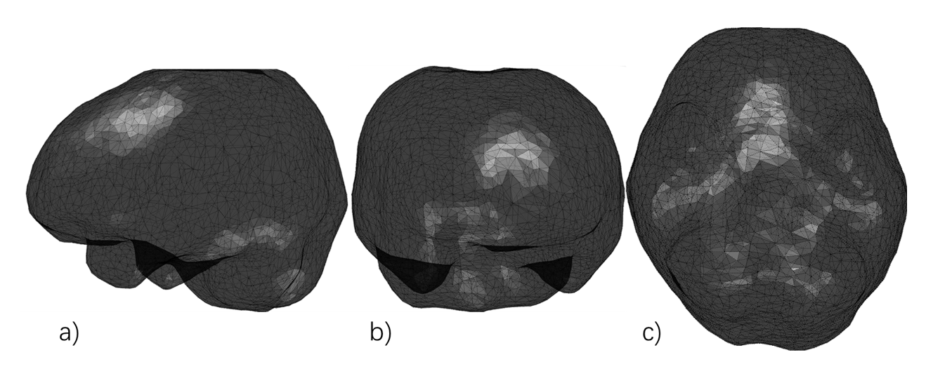
The background field satisfies the Laplace’s equation inside ROI.^2,6 This field with smooth surface can be solved using boundary condition in the integral equations as follow⁷:$$\begin{cases} \frac{1}{2}f_{\varGamma}\left( \boldsymbol{r}_{\varGamma} \right) =\iint_{\varGamma}{\left( G\left( \boldsymbol{r}_{\varGamma},\boldsymbol{r}_{\varGamma}\prime \right) \frac{\partial f_{\varGamma}\left( \boldsymbol{r}_{\varGamma}\prime \right)}{\partial n}-f_{\varGamma}\left( \boldsymbol{r}_{\varGamma}\prime \right) \frac{\partial G\left( \boldsymbol{r}_{\varGamma},\boldsymbol{r}_{\varGamma}\prime \right)}{\partial n} \right)}dS\prime\\ f\left( \boldsymbol{r} \right) =\iint_{\varGamma}{\left( G\left( \boldsymbol{r},\boldsymbol{r}\prime \right) \frac{\partial f_{\varGamma}\left( \mathbf{r}\prime \right)}{\partial n}-f_{\varGamma}\left( \boldsymbol{r}\prime \right) \frac{\partial G\left( \boldsymbol{r},\boldsymbol{r}\prime \right)}{\partial n} \right)}dS\prime\\\end{cases}，\begin{cases} \boldsymbol{r}_{\varGamma}\in \varGamma\\ \boldsymbol{r}\in M\\\end{cases}\,\, \left[ 1 \right] $$ Where M is the domain of ROI, Г is the surface of M, f is the background field inside M, r is the location where the field is observed, r′ is the location of the source point and n is the outer normal vector of Г. The function $$$G\left( \boldsymbol{r},\boldsymbol{r}\prime \right) =\frac{1}{4\pi \left| \boldsymbol{r}-\boldsymbol{r}\prime \right|}$$$ is the fundamental solution for the Poisson equation.⁷ In this study, the surface of brain is dispersed by a triangulation mesh. Fig.1 shows the mesh of the surface of brain. Using points located on the barycenter of the triangles on mesh as the discrete boundary elements and assuming that the boundary values within a triangular area are uniform, Eq.1 can be discretized as follow:$$\begin{cases} \frac{1}{2}f_{\varGamma i}\left( \boldsymbol{r} \right) =\sum_{j=1}^{N\,\,}{\left( \iint_{\varGamma j}{G\left( \boldsymbol{r}_{\varGamma i},\boldsymbol{r}_{\varGamma j}\prime \right) dS\prime} \right) \frac{\partial f_{\varGamma j}}{\partial n}-\left( \iint_{\varGamma j}{\frac{\partial G\left( \boldsymbol{r}_{\varGamma i},\boldsymbol{r}_{\varGamma j}\prime \right)}{\partial n}dS\prime} \right) f_{\varGamma j}}\\ f\left( \boldsymbol{r} \right) =\sum_{i=1}^{N\,\,}{\left( \iint_{\varGamma i}{G\left( \boldsymbol{r},\boldsymbol{r}_i\prime \right) dS\prime} \right) \frac{\partial f_{\varGamma i}}{\partial n}-\left( \iint_{\varGamma i}{\frac{\partial G\left( \boldsymbol{r},\boldsymbol{r}_i\prime \right)}{\partial n}dS\prime} \right) f_{\varGamma i}}\\\end{cases}\,\, \left[ 2 \right] $$ Where the Гi and Гj is the area of the triangular mesh and f_Гi and f_Гi is the boundary value of triangle i and j. Eq.2 can be formatted in a matrix form:$$\begin{cases} \boldsymbol{T}\prime\left( \frac{\partial \boldsymbol{f}_{\varGamma}}{\partial n} \right) =\left( \boldsymbol{Q}\prime+\frac{1}{2}\boldsymbol{I} \right) \boldsymbol{f}_{\varGamma}\\ \boldsymbol{f}=\boldsymbol{T}\left( \frac{\partial \boldsymbol{f}_{\varGamma}}{\partial n} \right) -\boldsymbol{Qf}_{\varGamma}\\\end{cases}\,\, \left[ 3 \right] \\\boldsymbol{T}_{i,j}^{\prime}\,\,=\,\,\iint_{\varGamma j}{G\left( \boldsymbol{r}_i,\boldsymbol{r}_{\mathrm{j}}\prime \right) dS\prime},\,\,\boldsymbol{Q}_{i,j}^{\prime}\,\,=\iint_{\varGamma j}{\frac{\partial G\left( \boldsymbol{r}_i,\boldsymbol{r}_{\mathrm{j}}\prime \right)}{\partial n}dS\prime}\\\boldsymbol{T}_{x,y,z,i}\,\,=\,\,\iint_{\varGamma i}{G\left( \boldsymbol{r}_{x,y,z},\boldsymbol{r}_{\mathrm{i}}\prime \right) dS\prime},\,\,\boldsymbol{Q}_{x,y,z,i}\,\,=\iint_{\varGamma i}{\frac{\partial G\left( \boldsymbol{r}_{x,y,z},\boldsymbol{r}_{\mathrm{i}}\prime \right)}{\partial n}dS\prime}\,\,$$ Where I is unit diagonal matrix. Based on Eq.3, a matrix L^-1 can be defined as $$$\boldsymbol{L}^{-1}=\boldsymbol{TT}\prime^{-1}\left( \boldsymbol{Q}\prime+\frac{1}{2}\boldsymbol{I} \right) -\boldsymbol{Q} $$$. The cost function of our method is formulated as follow:$$\underset{\,\, \left[ \begin{array}{c} \boldsymbol{\chi }\\ \boldsymbol{f}_{\boldsymbol{\varGamma }}\\\end{array} \right]}{\boldsymbol{\chi }=argmin}\,\,\left\| \boldsymbol{m}\cdot e^{i\left( \boldsymbol{D\chi }+\boldsymbol{L}^{-1}\boldsymbol{f}_{\boldsymbol{\varGamma }}\,\,-\,\,\boldsymbol{f}_{\boldsymbol{total}}\,\, \right)} \right\| _{2}^{2}+\lambda \left\| \boldsymbol{M}_G\boldsymbol{\nabla \chi } \right\| _1\,\, \left[ 4 \right] $$Where $$$\boldsymbol{\chi}$$$ is the local tissue susceptibility, m is weighting matrix,⁸ f_Г is the boundary value of background field, f_total is the total field, M_G is the binary edge mask and ▽ denotes the gradient operation.⁸

Methods

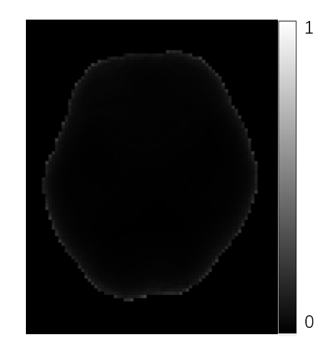
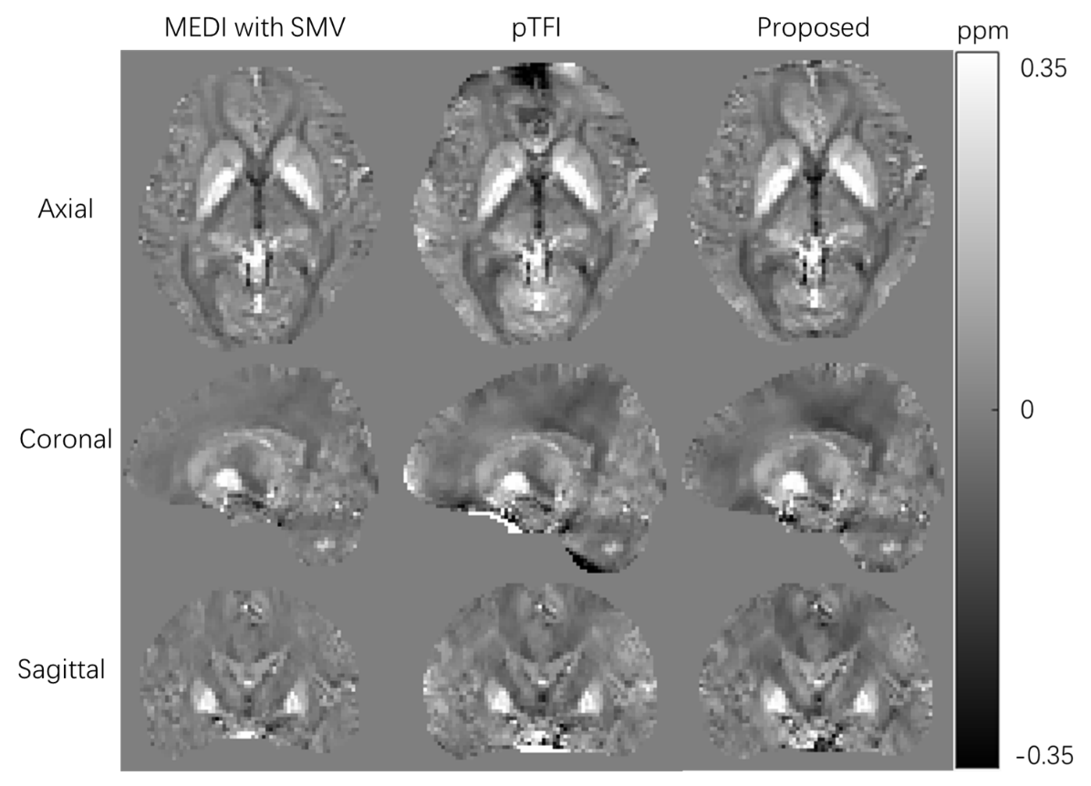
The following experiments were performed to validate the proposed method. We calculated the maximum absolute normalized inner product between the dipole kernel of local susceptibility and components of L^-1 for all background field boundary element inside ROI on a typical brain ROI segmented from an actual brain using the following formula:$$c\left( \boldsymbol{r}_{\mathrm{Local}} \right) =\max \left| \left< \boldsymbol{Mask}\cdot \boldsymbol{d}_{local},\left( \boldsymbol{L}^{-1} \right) _{i} \right> /\left( \left\| \boldsymbol{Mask}\cdot \boldsymbol{d}_{local} \right\| _2\cdot \left\| \left( \boldsymbol{L}^{-1} \right) _{i} \right\| _2 \right) \right|$$
We compared the susceptibility maps reconstructed by MEDI with SMV kernel,⁹ pTFI⁴ and our proposed method on in vivo brain data from a healthy subject. Scan parameters for QSM were as follows: TR/TE₁/ΔTE=36/6.2/5.1ms, voxel size=2×2×2 mm³ and bandwidth=240Hz/pixel. The total field map was obtained by nonlinear fitting of the multi-echo GRE data followed by graph cut based phase unwrapping.^9,10

Result

Fig.2 shows the good orthogonality between the background model and local dipole field in our method. Fig.3 shows the susceptibility maps reconstructed with three different methods. Our method had a good performance for background field removal. MEDI with SMV kernel suffers from a lack of low-frequency information. For pTFI method, parts of the background field were fitted as local field near the boundary.

Discussion

We have implemented the algorithm and obtained preliminary results in a low spatial resolution. The orthogonality between our background field model and local dipole kernel were numerically verified. Good performance of our method was achieved for background field removal on in vivo low-resolution images. Its performance has not been verified on high-resolution images because the L^-1 consists of four large scale dense matrixes. And there were still some artifacts in susceptibility map by our method, which may be caused by low precision of surface modeling. Those problems may be solved by using fast multipole method in further study.⁷

Conclusion

This work introduces a novel total field inversion method based on boundary element method. It is shown to have great performance for the separation between background field and local susceptibility.

Acknowledgements

No acknowledgement found.