4174

Quantitative comparison of DTI and STI principal eigenvectors

Nestor Munoz^1,2,3, Carlos Milovic^3,4, Christian Langkammer⁵, Sergio Uribe^2,3,6, and Cristian Tejos^1,2,3
¹Electrical Engineering, Pontificia Universidad Catolica de Chile, Santiago, Chile, ²Biomedical Imaging Center, Pontificia Universidad Catolica de Chile, Santiago, Chile, ³Millennium Institute for Intelligent Healthcare Engineering (iHEALTH), Santiago, Chile, ⁴School of Electrical Engineering, Pontificia Universidad Católica de Valparaiso, Valparaiso, Chile, ⁵Department of Neurology, Medical University of Graz, Graz, Austria, ⁶Department of Radiology, Pontificia Universidad Catolica de Chile, Santiago, Chile

Synopsis

Keywords: Susceptibility, Susceptibility

Diffusion Tensor Imaging (DTI) and Susceptibility Tensor Imaging (STI) are two MRI techniques that produces anisotropy information and fiber direction of biological tissue. For the brain, it has been suggested that both principal eigenvectors (PEV) point towards the same direction (i.e., direction of myelinated axons). However, different resolution of both techniques might produce differences in the PEVs. We proposed a quantitative method to compare DTI and STI PEVs based on the cosine of their angular difference. As expected, we found that PEVs from STI and DTI show similar directions in white matter and that consistency is lost for gray matter and CSF.

Introduction

Diffusion Tensor Imaging (DTI) is an MRI technique that uses diffusion properties of water to describe the magnitude, degree of anisotropy, and orientation of diffusion anisotropy of human tissues¹. Measurements of the DTI include the fractional anisotropy (FA) and principal eigenvectors (PEV)^1,2. PEV of DTI has shown to be parallel to the direction of the major diffusion, e.g., the white matter fiber in the brain³.
Susceptibility tensor imaging (STI) has recently appeared as an alternative MRI technique to study the anisotropy of biological tissue due to magnetic properties of the molecules⁴. In STI, the PEVs point to the most paramagnetic part of the eigenvalue, i.e., myelinated axons of white matter in the brain^5,6. As FA provides anisotropy information in diffusion images, the magnetic susceptibility anisotropy (MSA) of STI provides an image of anisotropy due to magnetic properties of the tissue^5,7–9.
In the case of the brain, it has been suggested that the principal eigenvectors of DTI and STI point towards the same direction (i.e., following the direction of myelinated axons)⁶. However, both images have different acquisition settings (e.g., different spatial resolution) that might generate different results in the images reconstructions. In this study we provide a quantitative analyze of the differences between DTI and STI principal eigenvectors.

Methods

A healthy volunteer was scanned in a 3T MR scanner (Prisma fit, Siemens) with a 20 channels head coil. For STI we acquired Gradient Recalled Echo (GRE) images at 9 different orientations with 4 echoes (4.57ms, 9.84ms, 14.76ms and 19.68ms); TR of 25ms; flip angle of 15°; FOV of 224x224x128 mm³; spatial resolution of 1mm³; and a total duration around 1.5 hours. For DTI we acquired DWI images with an Echo Planar protocol with SENSE of acceleration factor of 4; 103 different orientations with b-values between 5 and 1000 s/mm²; TE of 87.4ms; TR of 3.32s; FOV of 140x140x96; isotropic resolution of 1.5mm³. An anatomical T1-w GRAPPA image was acquired with TI of 900ms, TE of 2.7ms, TR of 1.9s FOV = 176x224x256 and resolution = 1mm³. All DWI and T1-w images were acquired with the subject in the same position.
Corregistration steps were made using flirt command from FSL^10–12. The T1-w image and all DWI images were corregistered to the GRE space. Segmentation of white matter (WM), gray matter (GM) and CSF was made by the fast algorithm of FSL. DTI reconstruction was made with the dtifit command in the GRE space. Each GRE echo orientation passed through a Laplacian unwrapping algorithm¹³; two background field removal: a Laplacian Boundary Value (LBV) ¹⁴ followed by a vSHARP background field removal¹⁵; and combination of echoes using MEDI toolbox^16–18 to obtain each local field map. Each orientation was corregistered to the image acquired parallel to the main magnetic field, and the STI was reconstructed using least squares estimation⁴. Finally, the angle θ between both principal eigenvectors was compared using the absolute value of their dot product:

$$|\cos(θ)|=|v_{1,DTI}, v_{1,STI}|$$

Results

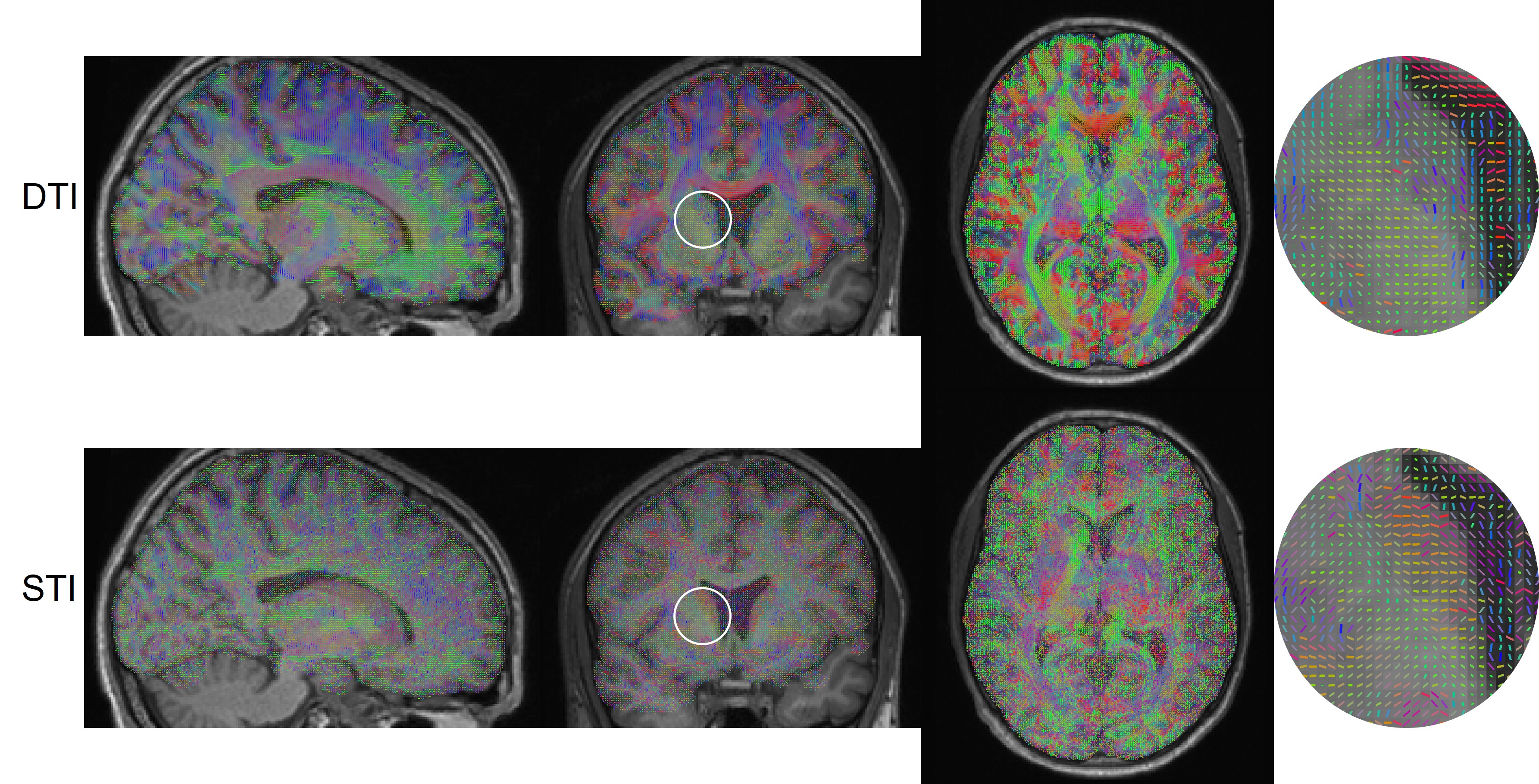
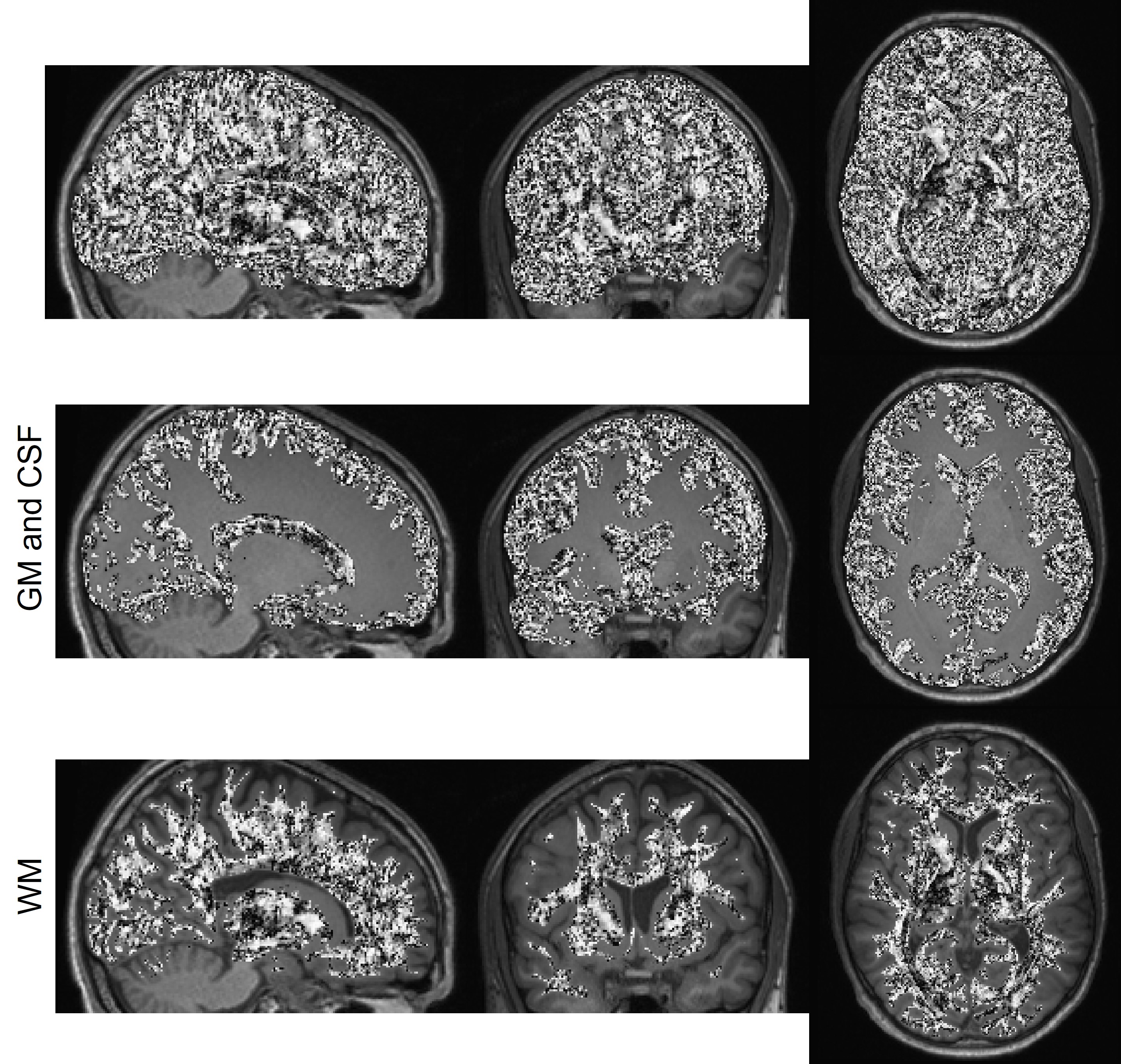
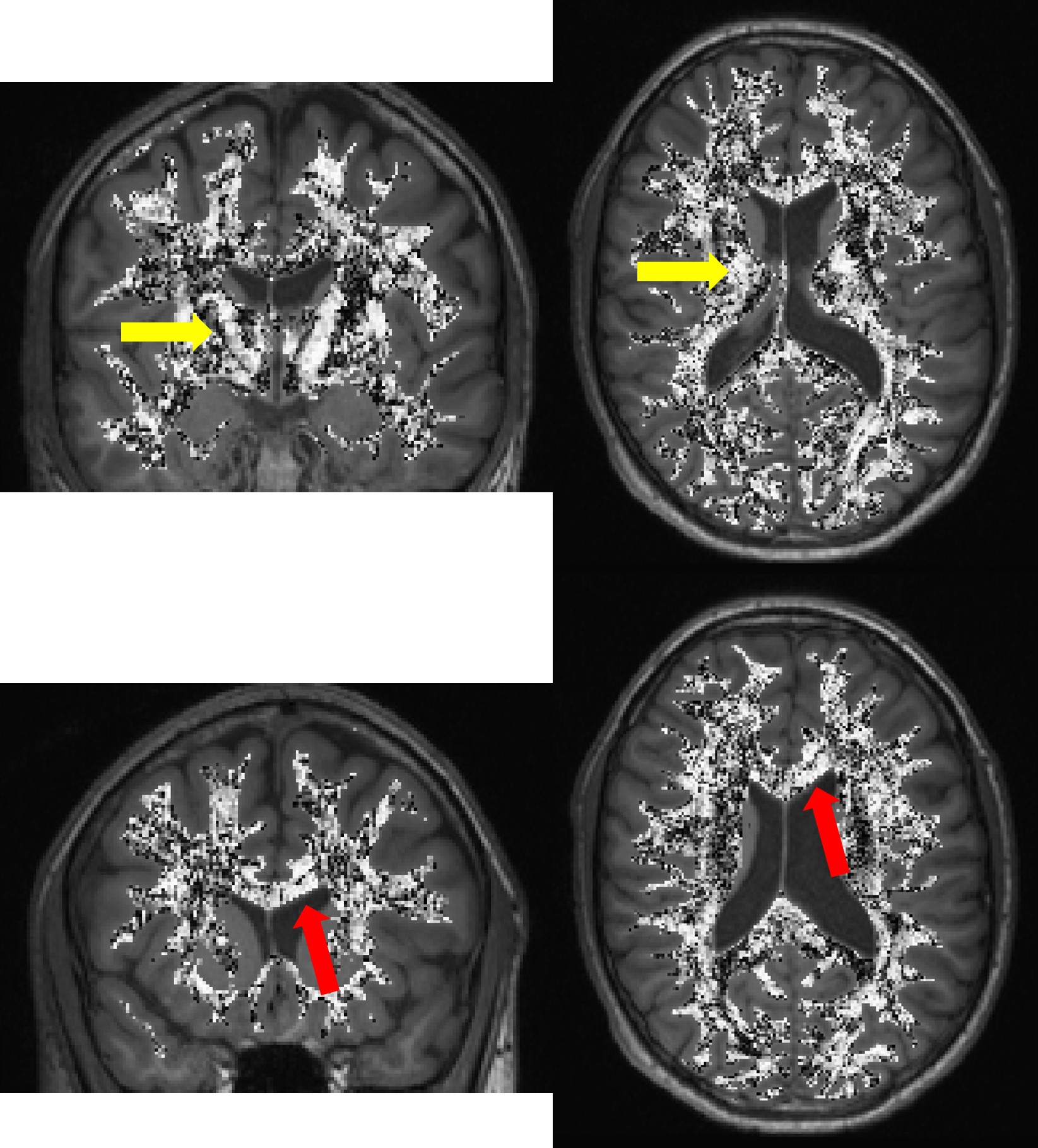
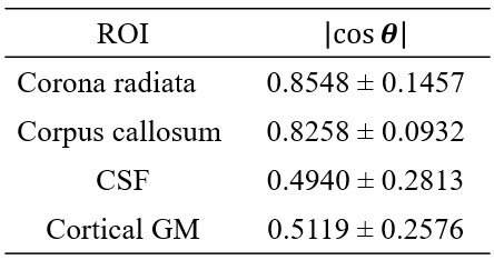
The PEV of DTI and STI images (after corregistration) are shown in figure 1, including a magnified view of the corona radiata, which is an area with highly organized axon fibers. Qualitatively, PEVs from STI and DTI show some similarities. Those similarities can be confirmed quantitatively, looking at their angle (i.e., their dot product) as shown in figure 2, masking those areas corresponding to WM, and those corresponding to GM and CSF. As expected, the $$$\cosθ$$$ shows values close to one in areas with highly organized axon fibers (e.g., the corona radiata and the corpus callosum³) and that value decreases for areas with more isotropic behavior (GM and CSF)³ as shown in figure 3. A summary of the cosine computed at different ROIs in these regions are shown in table 1.

Discussion

As expected, PEVs obtained from STI and DTI tend to point to the same direction. This is explained by the physical properties of the brain tissue: Myelinated axons diffuses more in the direction of the fiber; and magnetic susceptibility of the fibers is more paramagnetic in the same direction. However, principal eigenvectors from both DTI and STI are affected by noise, reconstruction errors and they are somehow affected by the interpolation (as a result of the up sampling or down sampling) when transforming the image resolution of one set to the other. This might explain the differences in the directions, and the fact that PEV from DTI images look smoother than those from STI images. These differences might also affect the accuracy of algorithms that use regularization procedures based on DTI information to reconstruct the susceptibility tensors (e.g., DRSTI¹⁹). Finally, our propose of using cosine of the angular differences between vectors is a viable quantitative method to compare DTI and STI.

Acknowledgements

This work has been funded by the following grants: Fondecyt 1191710 and 1231535, Anillo ACT912064, Millennium Institute for Intelligent Healthcare Engineering, iHEALTH (ICN2021_004), and the Austrian Science Fund (FWF grant numbers: P30134, P35887).

References

1. Hagmann P, Jonasson L, Maeder P, Thiran JP, Wedeen J van, Meuli R. Understanding Diffusion MR Imaging Techniques: From Scalar Diffusion-weighted Imaging to Diffusion Tensor Imaging and Beyond1. https://doi.org/101148/rg26si065510. 2006;26(SPEC. ISS.). doi:10.1148/RG.26SI065510

2. Basser PJ, Pierpaoli C. Microstructural and physiological features of tissues elucidated by quantitative-diffusion-tensor MRI. J Magn Reson B. 1996;111(3):209-219. doi:10.1006/JMRB.1996.0086

3. Alexander AL, Lee JE, Lazar M, Field AS. Diffusion tensor imaging of the brain. Neurotherapeutics. 2007;4(3):316. doi:10.1016/J.NURT.2007.05.011

4. Liu C. Susceptibility tensor imaging. Magn Reson Med. 2010;63(6):1471-1477. doi:10.1002/mrm.22482

5. Li W, Liu C, Duong TQ, van Zijl PCM, Li X. Susceptibility tensor imaging (STI) of the brain. NMR Biomed. 2017;30(4). doi:10.1002/nbm.3540

6. Liu C, Li W, Wu B, Jiang Y, Johnson GA. 3D fiber tractography with susceptibility tensor imaging. Neuroimage. 2012;59(2):1290-1298. doi:10.1016/j.neuroimage.2011.07.096

7. Xie L, Dibb R, Cofer GP, et al. Susceptibility tensor imaging of the kidney and its microstructural underpinnings. Magn Reson Med. 2015;73(3):1270-1281. doi:10.1002/mrm.25219

8. Wei H, Gibbs E, Zhao P, et al. Susceptibility tensor imaging and tractography of collagen fibrils in the articular cartilage. Magn Reson Med. 2017;78(5):1683-1690. doi:10.1002/mrm.26882

9. Wei H, Decker K, Nguyen H, et al. Imaging diamagnetic susceptibility of collagen in hepatic fibrosis using susceptibility tensor imaging. Magn Reson Med. 2020;83(4):1322-1330. doi:10.1002/MRM.27995

10. Jenkinson M, Beckmann CF, Behrens TEJ, Woolrich MW, Smith SM. FSL. Neuroimage. 2012;62(2):782-790. doi:10.1016/j.neuroimage.2011.09.015

11. Woolrich MW, Jbabdi S, Patenaude B, et al. Bayesian analysis of neuroimaging data in FSL. Neuroimage. 2009;45(1 Suppl). doi:10.1016/j.neuroimage.2008.10.055

12. Smith SM, Jenkinson M, Woolrich MW, et al. Advances in functional and structural MR image analysis and implementation as FSL. In: NeuroImage. Vol 23. ; 2004. doi:10.1016/j.neuroimage.2004.07.051

13. Schofield MA, Zhu Y. Fast phase unwrapping algorithm for interferometric applications. Opt Lett. 2003;28(14):1194-1196. doi:10.1364/ol.28.001194

14. Zhou D, Liu T, Spincemaille P, Wang Y. Background field removal by solving the Laplacian boundary value problem. NMR Biomed. 2014;27(3):312-319. doi:10.1002/nbm.3064

15. Kan H, Kasai H, Arai N, Kunitomo H, Hirose Y, Shibamoto Y. Background field removal technique using regularization enabled sophisticated harmonic artifact reduction for phase data with varying kernel sizes. Magn Reson Imaging. 2016;34(7):1026-1033. doi:10.1016/j.mri.2016.04.019

16. de Rochefort L, Brown R, Prince MR, Wang Y. Quantitative MR susceptibility mapping using piece-wise constant regularized inversion of the magnetic field. Magn Reson Med. 2008;60(4):1003-1009. doi:10.1002/MRM.21710

17. Kressler B, de Rochefort L, Liu T, Spincemaille P, Jiang Q, Wang Y. Nonlinear Regularization for Per Voxel Estimation of Magnetic Susceptibility Distributions from MRI Field Maps. IEEE Trans Med Imaging. 2010;29(2):273. doi:10.1109/TMI.2009.2023787

18. Liu T, Wisnieff C, Lou M, Chen W, Spincemaille P, Wang Y. Nonlinear formulation of the magnetic field to source relationship for robust quantitative susceptibility mapping. Magn Reson Med. 2013;69(2):467-476. doi:10.1002/MRM.24272

19. Bao L, Xiong C, Wei W, Chen Z, van Zijl PCM, Li X. Diffusion-regularized susceptibility tensor imaging (DRSTI) of tissue microstructures in the human brain. Med Image Anal. 2021;67. doi:10.1016/j.media.2020.101827

Figures

Figure 1. Principal eigenvectors of the STI and DTI images corregistered to the GRE space in three different anatomical views. First row shows the principal eigenvectors of diffusion images, and the second row shows the principal eigenvectors of susceptibility images. A zoomed view of the corona radiata is shown in both principal eigenvectors.

Figure 2. Absolute value of the cosine of the angle between the DTI and STI principal eigenvectors. Segmentation of gray matter and CSF is shown in the second row, and the segmentation of the third row is shown in the third row.

Figure 3. Coronal and axial view of the cosine of the angle in the regions of interest. First row shows images of the coronal radiata (yellow arrows), and the second row shows images of the corpus callosum (red arrows).

Table 1. Summary of equation 1 applied to ROIs the corona radiata and the corpus callosum.

Proc. Intl. Soc. Mag. Reson. Med. 31 (2023)

4174

DOI: https://doi.org/10.58530/2023/4174