Synopsis

Keywords: Susceptibility, Data Processing

A pipeline to reconstruct multiple resolution QSM data using a QSM network trained at a single resolution is proposed. The local field map is re-sampled multiple times in different spatial locations, and the re-sampled local field maps are used to reconstruct QSM maps at training data resolution. The reconstructed maps are then combined, and corrected for using a procedure named “dipole compensation”. When compared to two scenarios to reconstruct different resolution data using network trained at a single resolution, the proposed pipeline demonstrated the best performance both qualitatively and quantitatively.

Introduction

Deep learning algorithms for QSM have demonstrated great potentials.^1–5 However, it was reported that the deep learning methods fail to reconstruct data with resolution different from that of the training resolution.⁶ In this work, we propose a pipeline to reconstruct multiple resolution QSM data using QSMnet trained at a single resolution.

Methods

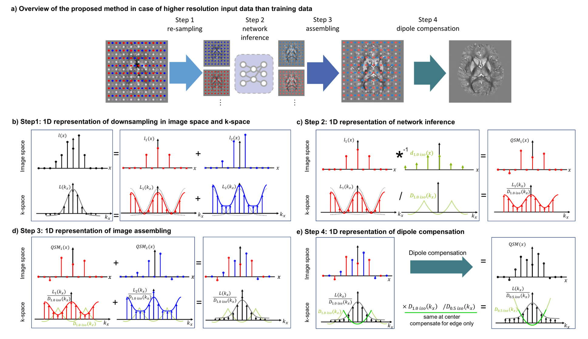
The proposed pipeline consists of four steps. Overview of the proposed method is displayed in Figure 1 for the case where input data is at a higher resolution (resol_input = 0.5 mm³) compared to that of the network training resolution (resol_train = 1.0 mm³). While the diagrams are represented in 1D for simplification, extension to 3D is straightforward.
[Step 1: re-sampling of local field map] First, the local field maps are re-sampled to the training resolution at multiple spatial locations (Figure 1b). This is analogous to multiplying comb functions with different shifts, which results in k-space aliasing with different linear phase for each case (red and blue cases in Figure 1b).
[Step 2: network inference] The re-sampled field maps can be input into the network. The network performs a dipole de-convolution in the image space; and a dipole division in the k-space, which is a pointwise operation (Figure 1c).
[Step 3: assembling] By assembling QSM maps of the red and blue sampling cases, an erroneous QSM can be reconstructed (Figure 1d). Because network inference is a pointwise division in the k-space, the resulting erroneous QSM is the k-space of the original local field map ($$$L(k_{x})$$$) divided by the replicated dipole kernel of 1.0 mm³ resolution ($$$D_{1.0 iso}(k_{x})$$$).
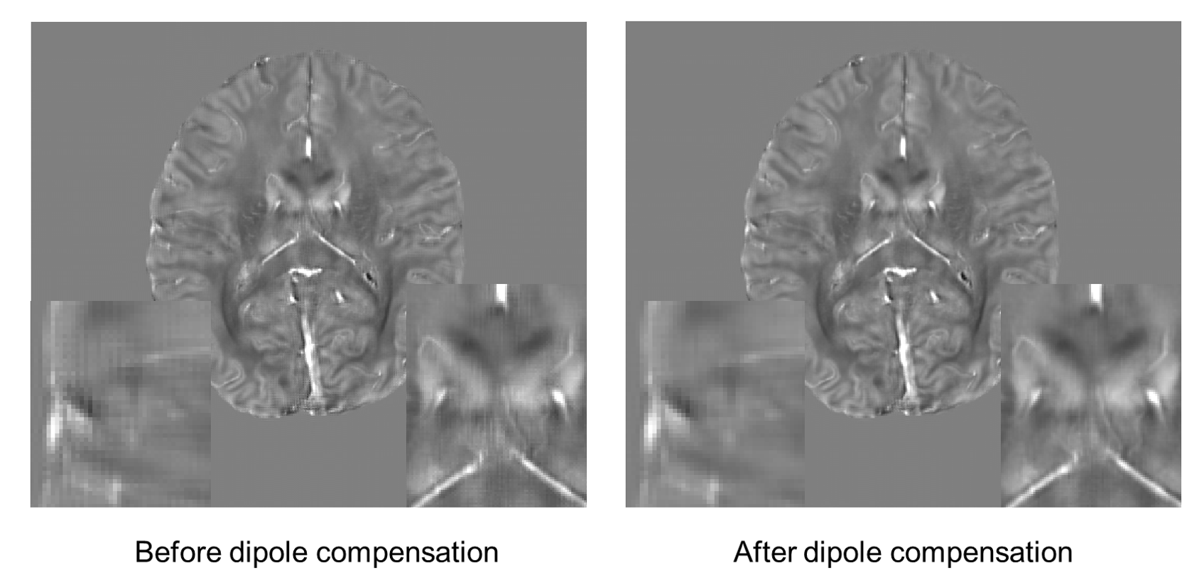
[Step 4: dipole compensation] The k-space of the desired QSM is $$$L(k_{x})$$$ divided by the dipole kernel of 0.5 mm³ resolution ($$$D_{0.5 iso}(k_{x})$$$). Because $$$D_{1.0 iso}(k_{x})$$$ and $$$D_{0.5 iso}(k_{x})$$$ are same at the center, this difference can be compensated by multiplying $$$D_{1.0 iso}(k_{x})/D_{0.5 iso}(k_{x})$$$ at the edge of the k-space. We call this procedure the dipole compensation (Figure 1e).
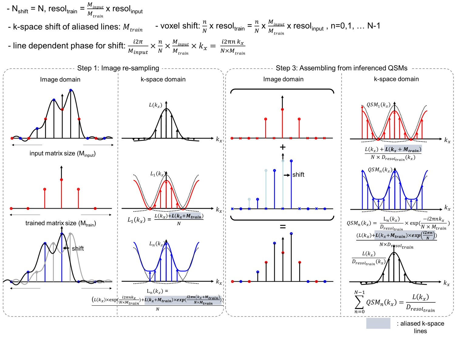
The method can be extended to non-integer resolution difference case by viewing the re-sampling of local field map as image shift and re-sampling (Figure 2). In the red sampling case, the local field map is directly undersampled, resulting in k-space aliasing.
$$L_1(k_x)=\frac{L(k_x)+L(k_x+M_{train})}{N}$$
Where $$$L_{1}(k_{x})$$$ is the k-space of the undersampled local field map and M_train is the matrix size of the data re-sampled to training resolution. The blue undersampling case can be seen as a combination of shifting and undersampling. Shift in image space is multiplying linear phase in k-space; Assuming sub-voxel shift in the training resolution ($$${n\over N}\times resol_{train}$$$, where n = 0,1, … N-1), each line of k-space is multiplied by a linear phase $$$\phi(k_x)=exp({i2\pi nk_x \over N \times M_{train}})$$$ before being aliased.
$$L_n(k_x)=\frac{L(k_x)\times{exp}(\frac{i2{\pi}nk_x}{N\times{M_{train}}})+L(k_x+M_{train})\times{exp}(\frac{i2{\pi}n(k_x+M_{train}}{N\times{M_{train}}})}{N}$$
After network inference, QSM from the blue sampling case is shifted back to the original position by multiplying an inverse linear phase $$$\phi(k_x)=exp({-i2\pi nk_x \over N \times M_{train}})$$$ in k-space.
$$QSM_n(k_x)=L_n(k_x)\times\frac{-i2{\pi}nk_x}{N\times{M_{train}}}=\frac{L(k_x)+L(k_x+M_{train}){\times}exp(\frac{i2{\pi}n}{N})}{N{\times}D_{resol_{train}}(k_x)}$$
Therefore, the aliased k-space lines cancel out when summed over the number of shift (N), leaving the erroneous QSM map subject to dipole compensation.
$$\sum_{n=0}^{N-1}{QSM_n(k_x)}=\frac{L(k_x)}{D_{resol_{train}}(k_x)}$$
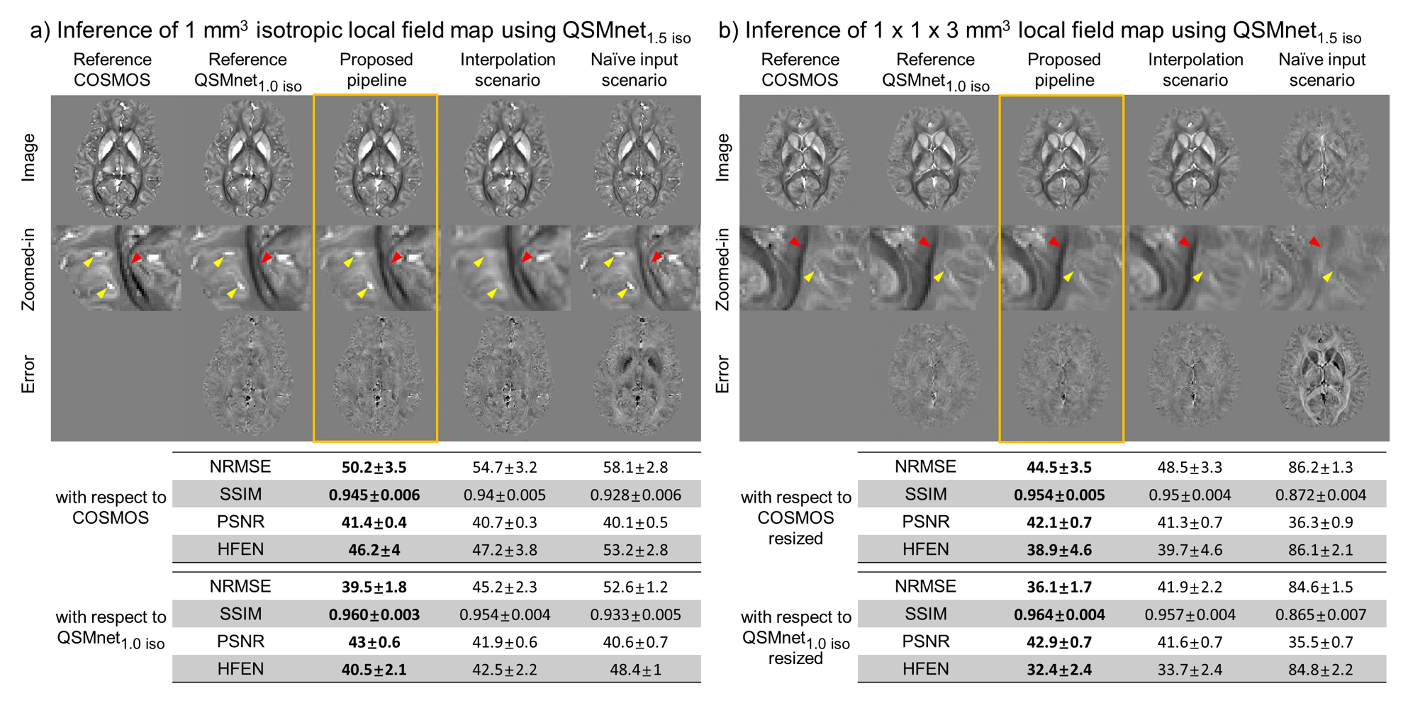
Data QSMnet dataset is used. For quantitative evaluation, we resized the QSMnet data by k-space cropping to 1.5 mm³ isotropic resolution for training. The original data (1 mm³ isotropic) and data resized to 1×1×3 mm³ resolution by k-space cropping were utilized as test data.
Network Training QSMnet_1.5iso was trained using 1.5 mm³ isotropic data from 7 subjects. For comparison, QSMnet_1.0iso was trained using 1.0 mm³ isotropic data of the same subjects.
Evaluation The proposed pipeline was compared with two scenarios: interpolation and naïve input. In the interpolation scenario, the local field map was resized to resol_train by cropping the k-space, and the resulting QSM was interpolated to resol_input. In case of naïve input, the local field map was naïvely input into the QSMnet without considering the resolution difference. The images were compared with COSMOS and QSMnet_1.0iso results both visually and quantitatively (NRMSE, SSIM, PSNR, HFEN). COSMOS and QSMnet_1.0iso results were resized to 1×1×3 mm³ resolution for evaluation of anisotropic data reconstruction.

Results

In both isotropic and anisotropic data, the proposed method provided the best reconstruction quality out of the three tested scenarios (Figure 3). In particular, in the zoomed-in images, small structures are diminished in the interpolation scenario (yellow arrowheads), while the white matter structures are flattened in the naïve input results (red arrowheads). These results are further supported by the quantitative results where the proposed method provided the best metrics compared to both COSMOS and QSMnet_1.0iso. The metrics computed with respect to QSMnet_1.0iso displays higher performance compared to that calculated with respect to COSMOS in both isotropic and anisotropic resolution. This is because the performance of the proposed method depends on the network performance. The effect of dipole compensation on the reconstructed QSM map is shown in Figure 4. The method can also be utilized to reconstruct positive and negative susceptibility maps using Chi-sepnet⁷ (Figure 5; abstract #7204).

Conclusion

The proposed method enables resolution-free QSM reconstruction using QSMnet trained at a single resolution. The resulting QSM maps preserve high-frequency details, and the quantitative metrics demonstrate high quality. In practice, trained QSMnet+ available online⁸ can be used to reconstruct QSM with arbitrary resolution.

Acknowledgements

This work was supported by Heuron Co. Ltd., and the BK21 FOUR program of the Education and Research Program for Future ICT Pioneers, Seoul National University in 2022.