Synopsis

Keywords: Electromagnetic Tissue Properties, Quantitative Susceptibility mapping

QSM is a promising MRI techniques that enables the assessment of magnetic properties of tissue. However, its underlying biophyisical source of contrast is still unknown. It has been shown that iron is well correlated in the basal ganglia, however this hasn't been investigates for other regions. Furthermore, iron can be presented in different forms in the brain, each one having different functions and properties. This work aims to assess the composition of brain structures regarding its paramagnetic ions' and total metal content, comparing their concentrations with magnetic susceptibility assessed by QSM

Introduction

Quantitative Susceptibility Mapping (QSM) has been vastly used to assess magnetic susceptibility changes in neurodegenerative diseases [1]. Previous studies showed that the source of contrast in regions of the basal ganglia are mostly correlated with total iron concentration [2], indicating QSM as an in vivo indirect iron quantification technique. However, the relationship between specific iron forms and QSM are not fully understood yet [3]. Furthermore, although in lower concentrations, paramagnetic copper appears in some biomolecules, which could also contribute to magnetic susceptibility. Here, we propose the use Electron Paramagnetic Resonance (EPR) technique to assess and quantify paramagnetic ions’ concentration within cerebral tissue of different brain regions [4] and compare with their respective magnetic susceptibility extracted by QSM and total metal concentration assessed by Inductive-Coupled Plasma Mass Spectrometry (ICP-MS).

Methods

Subjects were recruited from the Death Verification Service of the Capital in São Paulo and after obtaining informed consent from the family in situ MRI was performed right before autopsy at the Imaging Platform at the Autopsy Room of the Medical School of the University of São Paulo. No subjects presented history of neurological conditions. Four subjects (ages: 53, 56, 76 and 91 years; 2 males) were included in this study. MRI was performed on a 7T MRI scanner (Magnetom, SIEMENS) with a 32 receiver channel head coil (Nova Medical, USA). A multi-echo (n=5) gradient echo were acquired (1st TE/ΔTE = 5/4 ms; TR = 25ms; 0.5x0.5x1.0 res.).

Upon autopsy, whole brain was procured and fixed in buffered 10% formalin. After 3 years of fixation, brain tissue samples of several regions were extracted from the axial slices (1cm thick) by an experienced neuropathologist. A picture of each slice was taken, identifying the location of each extraction. Extracted samples (both sides) were: Caudate Nucleus (CN); Entorhinal Cortex (ENT); Globus Pallidus (GP); Hippocampus (HIP); Putamen (PUT); Red Nucleus (RN); Substantia Nigra (SN).

QSM maps were processed on Matlab (2021b) with the following pipeline: 1) coil combination using MCPC-3D-S; 2) echo combination using nonlinear fitting; 3) phase unwrapping using PRELUDE; 4) Background field removal using PDF; 5) dipole inversion using MEDI-L1. ROIs were manually segmented using ITK-SNAP by visual comparison with pictures taken during sample extraction.

Tissue samples were weighted before (wet mass) and after lyophilization (dry mass). EPR spectra were recorded on dried samples in a X-Band equipment, and processed using EasySpin toolbox. Relative concentrations of each paramagnetic site were estimated following the pipeline described in [4]. Metal concentrations of $$$^{55}Mn$$$, $$$^{27}Al$$$, $$$^{66}Zn$$$, $$$^{63}Cu$$$ and $$$^{56}Fe$$$ were measured by ICP-MS.

Two general linear models (GLM) were applied involving all the subjects/regions and considering $$$\chi$$$ as dependent variable and ICP-MS (Model 1) and EPR (Model 2) as independent variables. Correlation tests were also applied for EPR, ICP-MS and , considering a threshold of p=0.05 for significant correlations.

Model 1: $$$\chi = C_0 + C_{Fe}[^{56}Fe] + C_{Cu}[^{63}Cu] + C_{Zn}[^{66}Zn] + C_{Mn}[^{55}Mn] + C_{Al}[^{27}Al]$$$

Model 2: $$$\chi = C_0 + C_{g=4.3}[EPR_{g=4.3}] + C_{g=2.0}[EPR_{g=2.0}] + C_{Cu}[EPR_{Cu}] + C_{OR}[EPR_{OR}]$$$

Results/Discussion

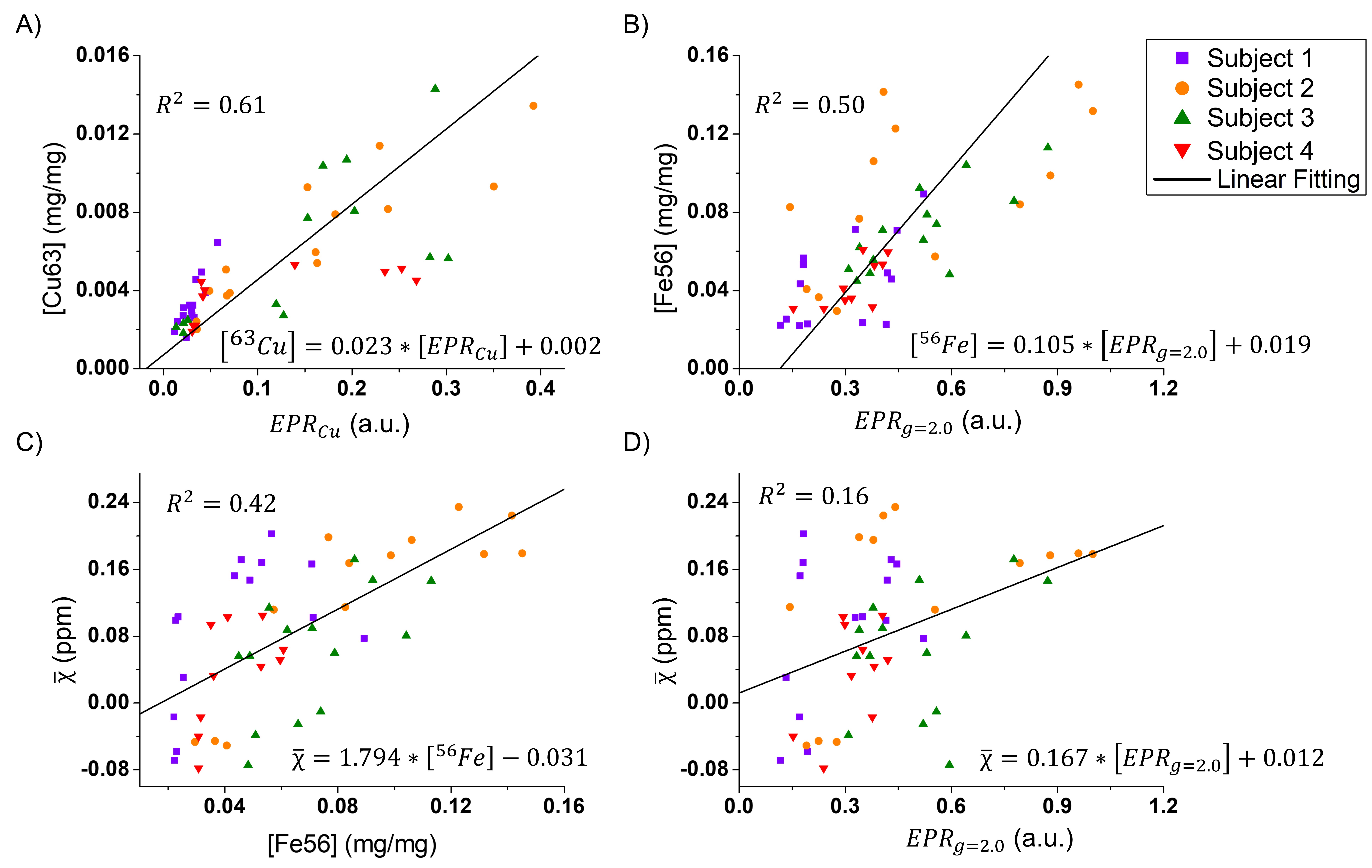
The EPR spectra of all subjects showed four main paramagnetic sites: a peak at $$$g = 4.3$$$ ($$$EPR_{g=4.3}$$$), a peak with anisotropic g-factor ($$$g_{\perp} = 2.05$$$ and $$$g_{||} = 2.25$$$) related to copper ions ($$$EPR_{Cu}$$$), a broad peak centered at $$$g = 2.0$$$ ($$$EPR_{g=2.0}$$$) [4] and a fourth narrow peak at $$$g = 1.9839$$$ associated to an organic radical ($$$EPR_{OR}$$$).

GLM analysis showed that for Model 1 only $$$[^{56}Fe]$$$ was significant, and for Model 2 only $$$[EPR_{g=2.0}]$$$ was significant.

Figure 1 shows the significant correlations between EPR, ICP-MS and $$$\chi$$$. Results from Figure 1.A and 1.B indicates that these EPR peaks are well correlated to $$$^{63}Cu$$$ and $$$^{56}Fe$$$, respectively. Figure 1.C is in agreement to literature, and supports the ideia that iron is the major contributor to $$$\chi$$$. FInally, although $$$EPR_{g=2.0}$$$ correlated to $$$\chi$$$, the low R indicates that this peak alone is not able to explain the susceptibility contrast.

On a previous study [4], $$$EPR_{g=2.0}$$$ was found to have an antiferromagnetic contribution and a magnetic behaviour with temperature similar to purified ferritin (although not exactly the same). This supports the idea of $$$EPR_{g=2.0}$$$ being related to iron, and possibly to ferrihydrite cores of ferritin.

A limitation of this study is the low number of subjects. By increasing the number of subjects, analysis for each ROI individually would give further insights. Furthermore, it is known that ex situ differs from in situ conditions, therefore ex situ images should also be used. Future studies should also include ex situ images for comparison. Finally, while very sensitive to paramagnetic ions, EPR can only detect unpaired electrons, which restricts the ionic species it can detect. Complementary measurements should also be used to improve the results observed here.

Conclusion

We demonstrated the applicability of EPR to study different paramagnetic ions in brain samples, which can be used to infer possible sources of contrast mechanism observed in QSM. Results from ICP-MS showed that $$$[^{56}Fe]$$$ is well correlated to QSM in agreement with other studies. Results from EPR indicates that only $$$EPR_{g=2.0}$$$, which is thought to be related to ferritin, correlates with QSM, however it should be noted the low R value.

Acknowledgements

The authors thanks the funding agencies that supported this study: São Paulo Research Foundation (FAPESP, project: 2015/10305–3), Brazilian National Council for Scientific and Technological Development (CNPq, project: 427977/2018–5 and F.S.O. fellowship), National Institute of Health (NIH) for R01AG070826 grant, and Coordenação de Aperfeiçoamento de Pessoal de Nível Superior – Brasil (CAPES) for financial support.