4151
Effective axon radii across the human corpus callosum for a group of subjects: comparability between MRI and histology1Institute of Systems Neuroscience, University Medical Center Hamburg-Eppendorf, Hamburg, Germany, 2Department of Neurophysics, Max Planck Institute for Human Cognitive and Brain Sciences, Leipzig, Germany, 3Paul Flechsig Institute - Center of Neuropathology and Brain Research, Medical Faculty University of Leipzig, Leipzig, Germany, 4Felix Bloch Institute for Solid State Physics, Faculty of Physics and Earth Sciences, Leipzig University, Leipzig, Germany, Leipzig, Germany
Synopsis
Keywords: Diffusion/other diffusion imaging techniques, Validation, Histology Connectome Axon radius Deep learning
Robust MRI-based axon radius estimation is sensitive to a tail-weighted estimate of the ensemble-average axon radius, i.e., the effective axon radius ($$$r_{eff}$$$). Existing validation studies of $$$r_{eff}$$$ in the human brain are confounded because the histological gold standard cannot representatively sample the tail of the axon radii distribution due to limited sample size. We compare in vivo, MRI-based $$$r_{eff}$$$ of five healthy adults against a representative histological gold standard of three donors in the human corpus callosum and demonstrate that spatial patterns of the $$$r_{eff}$$$ along the anterior-posterior axis agree between in vivo MRI and ex vivo histology.Introduction
The axon radius is a major determinant of the conduction velocity of neuronal action potentials 1,2. Diffusion-weighted MRI (dMRI) can non-invasively characterize the axon radii distribution within an MRI voxel in terms of a tail-weighted effective MR axon radius 3,4 $$$r_{eff} = ^4\sqrt{(<r^6>/<r^2>)}$$$. Despite the strong weighting towards large axon radii, $$$r_{eff}$$$ has been shown to be a sensitive metric in the human brain 5. However, it is still necessary to validate the specificity of $$$r_{eff}$$$ against a histological gold standard. In particular, the histological gold standard for validation of the tail-weighted $$$r_{eff}$$$ requires a large field of view to sample the tail of the axon radii distribution 6, which is not given in existing validation studies 4,7-9 for the human brain. Here, we compare MRI-based $$$r_{eff}$$$ of five healthy adults against a large-scale histological gold standard 10 of three donors in the human corpus callosum. We investigate the agreement between spatial patterns of $$$r_{eff}$$$ in the corpus callosum between in vivo MRI and ex vivo histology and discuss confounding factors for direct comparison.Materials and Methods
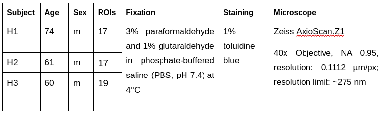
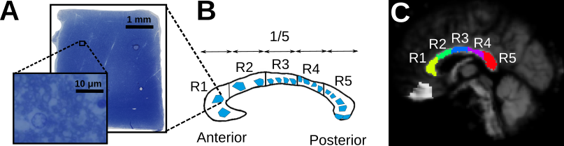
Histology Image Acquisition:We obtained three human corpus callosum samples (denoted as H1 to H3) at autopsy with prior informed consent and approval by the responsible authorities (Approvals #205/17-ek and #WF-74/16). We followed standard Brain Bank procedures for tissue processing and acquired large-scale light microscopy (lsLM) images (Figure 1A) for several ROIs. See Table 1 for details.
Histology Image Processing:
$$$r_{eff}$$$ were estimated per ROI from histology images in 10.
MRI Image Acquisition:
We acquired in vivo, diffusion-weighted MRI images of five healthy adult subjects (denoted as M1 to M5; age: 31 +- 3 years; sex: 2 male, 3 female) on a Siemens Connectome 3T scanner at MPI-CBS, Leipzig, Germany. We followed the robust protocol described in 5 i.e, in short: we applied b = [0.5 1, 2.5, 6, 30] ms/µm² for gradient directions [30, 30, 30, 120, 240] with variable gradient diffusion amplitude and a resolution of 2.5 × 2.5 × 2.5 mm3. Additionally, we acquired non-diffusion-weighted images for geometric susceptibility correction with the same (N=23) and reverse (N=10) phase encoding direction.
MRI Image Processing:
We preprocessed dMRI images withn an MRtrix3-based 11 pipeline using: denoising 12; Gibbs ringing artifact correction 13; geometric susceptibility, eddy current and motion correction 14-15; Rician bias correction 16-17. For $$$b <= 2.5 ms/μm^2$$$, we estimated DTI tensors and mapped fractional anisotropy (FA). For $$$b >= 6 ms/μm^2$$$, we estimated $$$r_{eff}$$$ using 18 after spherical averaging per $$$b$$$-value.
MRI image registration:
We transformed $$$r_{eff}$$$ maps to MNI space using SPM12 19: we first coregistered the average non-diffusion weighted image and T1-weighted MPRAGE image, then used the T1-weighted images for DARTEL registration 20 to MNI space.
Analyses:
We studied differences between acquisition methods (i.e., MRI and histology), subjects and regions within the corpus callosum. For the latter, we manually defined five equi-length regions as described in Figure 1B-C. To avoid partial volume effects in $$$r_{eff}$$$ introduced during normalization to MNI space, we considered only voxels with an across-subject average FA >= 0.7.
Results
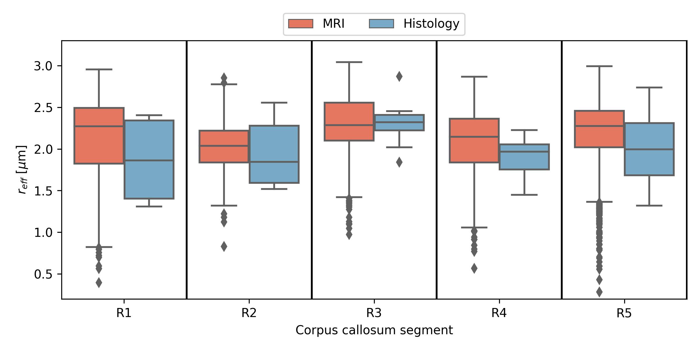
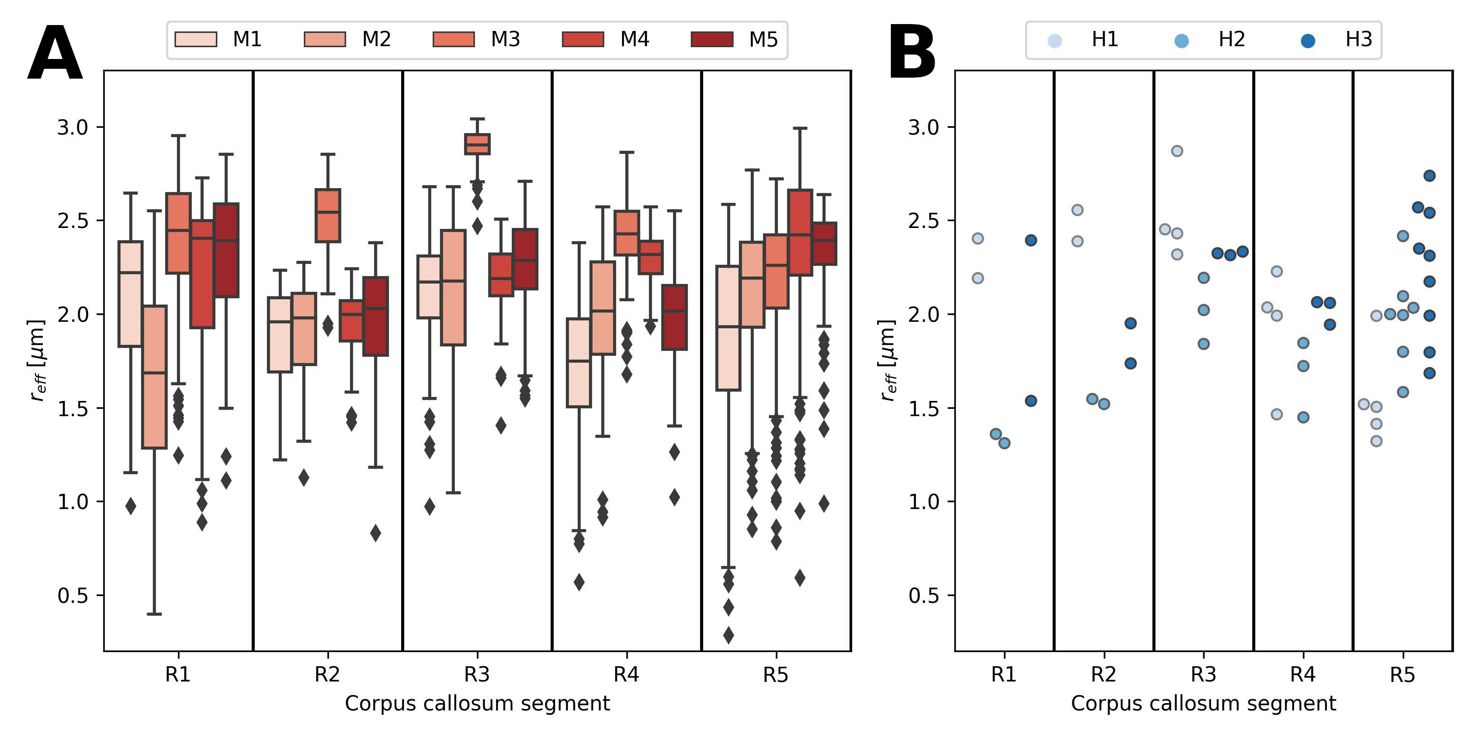
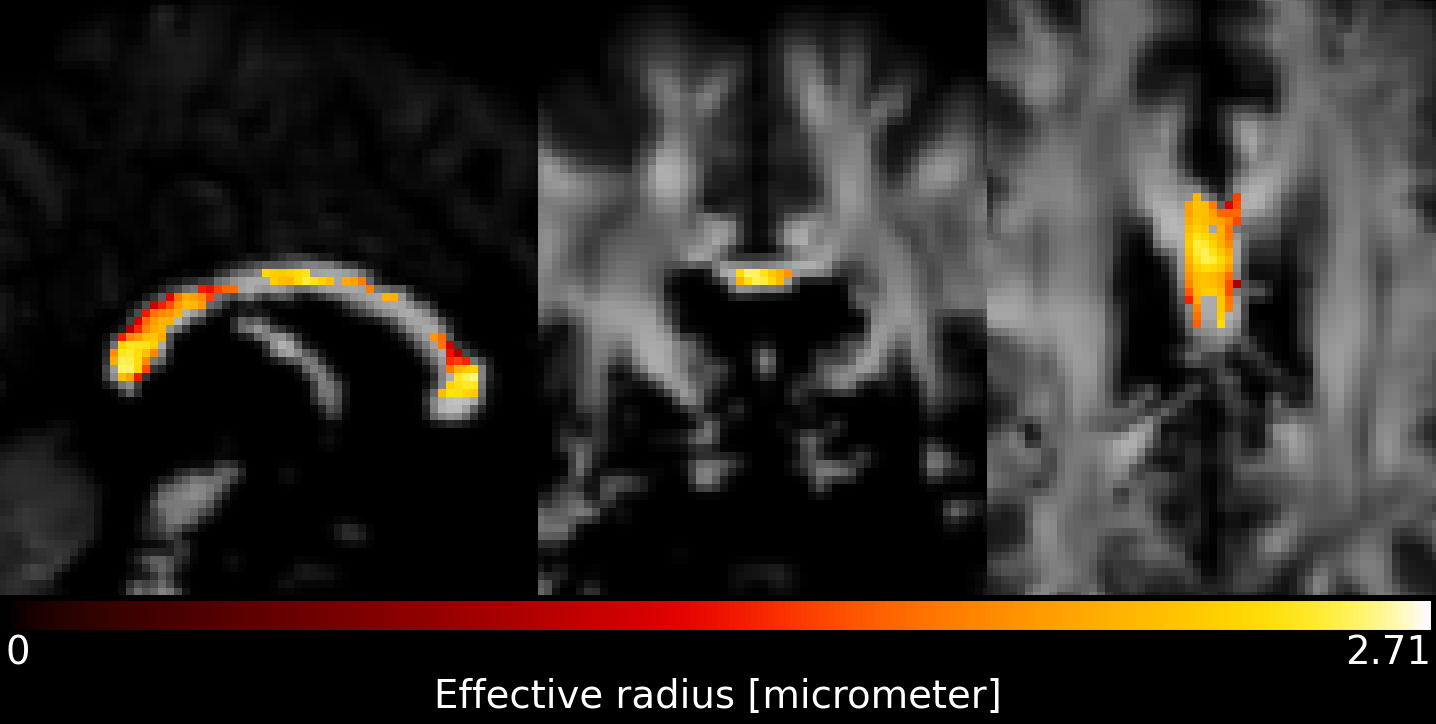
When pooling $$$r_{eff}$$$ across subjects (see Figure 2), the median $$$r_{eff}$$$ values in MRI were mostly higher than in histology across corpus callosum regions. MRI-based $$$r_{eff}$$$ follow an alternating high-low pattern moving from anterior to posterior regions in the corpus callosum, which resembled histology when discarding region R1. The spread of $$$r_{eff}$$$ for different regions was similar in MRI but not in histology. At the subject level (Figure 3), the alternating high-low pattern observed on the pooled data can be identified fully (M1 and M5 in MRI) or partially (M2 and M4 in MRI; H2 and H3 in histology) for individual subjects. The large spread of $$$r_{eff}$$$ for some regions in the subject-pooled data is reflected for individual subjects, i.e., in particular region R5. Figure 4 shows the across-subject, voxel-wise mean MR $$$r_{eff}$$$ within the corpus callosum.Discussion and Conclusion
We compared in vivo MRI-based effective radius ($$$r_{eff}$$$) against a large-scale histological gold standard and demonstrated that spatial patterns along the anterior-posterior axis of the corpus callosum are similar. However, one-to-one comparison across different subjects between in vivo MRI and ex vivo histology remains challenging because there are several potential sources of errors in both MRI- and histology-based $$$r_{eff}$$$. We expect main sources of biases in $$$r_{eff}$$$ in our study to be partial volume effects in MRI due to the transformation to MNI space and tissue shrinkage in histology; hence, we believe both MRI- and histology-based $$$r_{eff}$$$ are underestimated. Both biases, however, can be reduced: MRI-based $$$r_{eff}$$$ can be evaluated in subject space; histology-based $$$r_{eff}$$$ can be corrected by inverse-scaling with a tissue shrinkage factor assuming uniform tissue shrinkage 24. The different variability of $$$r_{eff}$$$ in histology and MRI across subjects and regions may have several sources. While the spatial smoothing in several MRI processing and registration steps may attenuate the true variability of $$$r_{eff}$$$, the variability of $$$r_{eff}$$$ in histology may reflect the smaller sample size but also the heterogeneity of subjects in terms of age when compared to MRI subjects. In total, the spatial agreement of $$$r_{eff}$$$ measured with different modalities encourages further in vivo application of the method.Acknowledgements
The research leading to these results has received funding from the European Research Council under the European Union's Seventh Framework Programme (FP7/2007-2013) / ERC grant agreement n° 616905.This work was supported by the German Research Foundation (DFG Priority Program 2041 "Computational Connectomics”, [MO 2397/5-1; MO 2397/5-2], by the Emmy Noether Stipend: MO 2397/4-1; MO 2397/4-2) and by the BMBF (01EW1711A and B) in the framework of ERA-NET NEURON and the Forschungszentrums Medizintechnik Hamburg (fmthh; grant 01fmthh2017).References
[1] S. G. Waxman, “Determinants of conduction velocity in myelinated nerve fibers,” Muscle Nerve, vol. 3, no. 2, pp. 141–150, 1980, doi: https://doi.org/10.1002/mus.880030207.
[2] M. Drakesmith, R. Harms, S. U. Rudrapatna, G. D. Parker, C. J. Evans, and D. K. Jones, “Estimating axon conduction velocity in vivo from microstructural MRI,” NeuroImage, vol. 203, p. 116186, Dec. 2019, doi: 10.1016/j.neuroimage.2019.116186.
[3] L. M. Burcaw, E. Fieremans, and D. S. Novikov, “Mesoscopic structure of neuronal tracts from time-dependent diffusion,” NeuroImage, vol. 114, pp. 18–37, Jul. 2015, doi: 10.1016/j.neuroimage.2015.03.061.
[4] J. Veraart et al., “Noninvasive quantification of axon radii using diffusion MRI,” eLife, vol. 9, p. e49855, Feb. 2020, doi: 10.7554/eLife.49855.
[5] J. Veraart, E. P. Raven, L. J. Edwards, N. Weiskopf, and D. K. Jones, “The variability of MR axon radii estimates in the human white matter,” Hum. Brain Mapp., vol. 42, no. 7, pp. 2201–2213, 2021, doi: 10.1002/hbm.25359.
[6] L. Mordhorst et al. Reliable estimation of the MRI-visible effective axon radius using light microscopy: the need for large field-of-views. Proc. Intl. Soc. Mag. Reson. Med. 30. 2021
[7] D. C. Alexander et al., “Orientationally invariant indices of axon diameter and density from diffusion MRI,” NeuroImage, vol. 52, no. 4, pp. 1374–1389, Oct. 2010, doi: 10.1016/j.neuroimage.2010.05.043.
[8] A. Horowitz, D. Barazany, I. Tavor, M. Bernstein, G. Yovel, and Y. Assaf, “In vivo correlation between axon diameter and conduction velocity in the human brain,” Brain Struct. Funct., vol. 220, no. 3, pp. 1777–1788, May 2015, doi: 10.1007/s00429-014-0871-0.
[9] G. M. Innocenti, R. Caminiti, and F. Aboitiz, “Comments on the paper by Horowitz et al. (2014),” Brain Struct. Funct., vol. 220, no. 3, pp. 1789–1790, May 2015, doi: 10.1007/s00429-014-0974-7.
[10] L. Mordhorst et al., “Towards a representative reference for MRI-based human axon radius assessment using light microscopy,” NeuroImage, vol. 249, p. 118906, Apr. 2022, doi: 10.1016/j.neuroimage.2022.118906.
[11] J.-D. Tournier et al., “MRtrix3: A fast, flexible and open software framework for medical image processing and visualisation,” NeuroImage, vol. 202, p. 116137, Nov. 2019, doi: 10.1016/j.neuroimage.2019.116137.
[12] J. Veraart, E. Fieremans, and D. S. Novikov, “Diffusion MRI noise mapping using random matrix theory,” Magn. Reson. Med., vol. 76, no. 5, pp. 1582–1593, 2016, doi: 10.1002/mrm.26059.
[13] E. Kellner, B. Dhital, V. G. Kiselev, and M. Reisert, “Gibbs-ringing artifact removal based on local subvoxel-shifts,” Magn. Reson. Med., vol. 76, no. 5, pp. 1574–1581, 2016, doi: 10.1002/mrm.26054.
[14] J. L. R. Andersson and S. N. Sotiropoulos, “An integrated approach to correction for off-resonance effects and subject movement in diffusion MR imaging,” NeuroImage, vol. 125, pp. 1063–1078, Jan. 2016, doi: 10.1016/j.neuroimage.2015.10.019.
[15] J. L. R. Andersson, M. S. Graham, E. Zsoldos, and S. N. Sotiropoulos, “Incorporating outlier detection and replacement into a non-parametric framework for movement and distortion correction of diffusion MR images,” NeuroImage, vol. 141, pp. 556–572, Nov. 2016, doi: 10.1016/j.neuroimage.2016.06.058.
[16] C. G. Koay and P. J. Basser, “Analytically exact correction scheme for signal extraction from noisy magnitude MR signals,” J. Magn. Reson., vol. 179, no. 2, pp. 317–322, Apr. 2006, doi: 10.1016/j.jmr.2006.01.016.
[17] B. Ades-Aron et al., “Evaluation of the accuracy and precision of the diffusion parameter EStImation with Gibbs and NoisE removal pipeline,” NeuroImage, vol. 183, pp. 532–543, Dec. 2018, doi: 10.1016/j.neuroimage.2018.07.066.
[18] J. Veraart, “AxonRadiusMapping.” Accessed: Nov. 09, 2022. [Online]. Available: https://github.com/NYU-DiffusionMRI/AxonRadiusMapping
[19] K. Friston, “CHAPTER 2 - Statistical parametric mapping,” in Statistical Parametric Mapping, K. Friston, J. Ashburner, S. Kiebel, T. Nichols, and W. Penny, Eds. London: Academic Press, 2007, pp. 10–31. doi: 10.1016/B978-012372560-8/50002-4.
[20] J. Ashburner, “A fast diffeomorphic image registration algorithm,” NeuroImage, vol. 38, no. 1, pp. 95–113, Oct. 2007, doi: 10.1016/j.neuroimage.2007.07.007.
[21] S. F. Witelson, “Hand and sex differences in the isthmus and genu of the human corpus callosum. A postmortem morphological study,” Brain J. Neurol., vol. 112 ( Pt 3), pp. 799–835, Jun. 1989, doi: 10.1093/brain/112.3.799.
[22] U. Bürgel, K. Amunts, L. Hoemke, H. Mohlberg, J. M. Gilsbach, and K. Zilles, “White matter fiber tracts of the human brain: three-dimensional mapping at microscopic resolution, topography and intersubject variability,” NeuroImage, vol. 29, no. 4, pp. 1092–1105, Feb. 2006, doi: 10.1016/j.neuroimage.2005.08.040.
[23] M. Jenkinson, C. F. Beckmann, T. E. J. Behrens, M. W. Woolrich, and S. M. Smith, “FSL,” NeuroImage, vol. 62, no. 2, pp. 782–790, Aug. 2012, doi: 10.1016/j.neuroimage.2011.09.015.
[24] T.Streubel, et al. "Quantification of tissue shrinkage due to formalin fixation of entire post-mortem human brain." Proc. Intl. Soc. Mag. Reson. Med. 29. 2020
Figures