Synopsis

Keywords: Image Reconstruction, Machine Learning/Artificial Intelligence

Deep learning methods have achieved superior reconstruction results in MRI reconstruction. Recently, denoising diffusion probabilistic models (DDPM) have demonstrated great potential in image-processing tasks. In this study, we combine denoising diffusion probabilistic models (DDPM) and GRAPPA for highly accelerated 3D imaging. The method sequentially performs DDPM and GRAPPA with specially designed sampling masks such that the benefits of the diffusion model and the availability of multi-channel data can be utilized jointly. Our results demonstrate that the proposed method can achieve an acceleration factor of up to 16 which is the product of the factors achieved by DDPM and GRAPPA alone.

Introduction

In the past few years, many deep learning fast MRI methods have achieved promising performance^1,2. Most methods are based on the convolutional neural network (CNN), which is a rather simple model with a shift-invariant filter. Recently, denoising diffusion probabilistic models (DDPM) have been proposed to improve the performance of the existing deep learning models for image reconstruction problems^3,4,5. However, a more comprehensive study in practical settings is still lacking. In this study, we investigate the integration of DDPM and GRAPPA for multi-channel 3D knee imaging. The integration allows a high acceleration factor that is the product of the factors achieved by DDPM and GRAPPA individually. A 2D undersampling pattern is specially designed for such integration. The performance is evaluated using 3D Dual-Echo Steady-State (DESS) knee images and shows its improvement over the integration of conventional CNN with GRAPPA.

Method

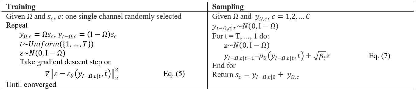
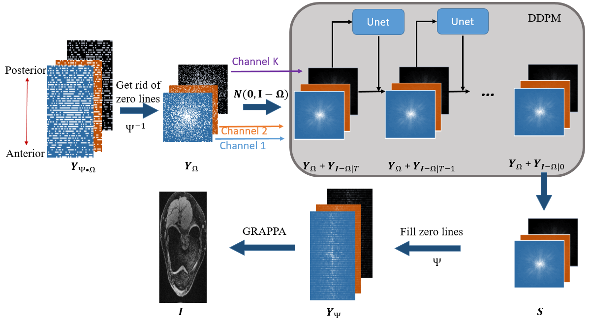
For acceleration, the undersampled k-space data $$$ \textbf{Y}_{\Psi\cdot\Omega}$$$ are acquired with a specially designed pattern, which can be represented as an integration of two under-sampling operators $$$\Psi$$$ and $$$\Omega$$$. The first operator $$$\Psi$$$ uniformly under-samples k-space by a factor of $$$\psi$$$ in the phase-encoding direction (1D-GRAPPA under-sampling), the second operator $$$\Omega$$$ randomly under-samples the remaining data by a factor of $$$\omega$$$ after $$$\Psi$$$ in phase and slice-encoding directions, result in total acceleration reduction is $$$\psi\times\omega$$$.
We perform DDPM and GRAPPA sequentially on $$$\textbf{Y}_{\Psi\cdot\Omega}$$$, as shown in Fig.1. First, zero-valued phase-encoding lines (i.e., the missing lines in GRAPPA) are eliminated in $$$\textbf{Y}_{\Psi\cdot\Omega}$$$ for all channels, resulting in k-space data $$$\textbf{Y}_{\Omega}$$$. We defined $$$y_{\Omega,c}=\Omega s_{c}$$$ and $$$y_{I-\Omega,c}=(I-\Omega) s_{c}$$$ as sampled and non-sampled k-space data for each channel, where $$$s_{c}$$$ is the full k-space data for the reduced field of view (FOV) image of channel $$$c=1,2...C$$$. We reconstruct each $$$s_{c}$$$ with data distribution of $$$s_{c}\sim q(s_{c})$$$ using DDPM. The reconstruction task is to estimate $$$q(s_{c}|y_{\Omega,c})$$$ only based on the undersampled k-space data $$$y_{\Omega,c}$$$. Since $$$y_{\Omega,c}$$$ is known and $$$s_{c}=y_{\Omega,c}+y_{I-\Omega,c}$$$, the problem is equivalent to estimating $$$q(y_{I-\Omega,c}|y_{\Omega,c})$$$.
The main idea of DDPM is that if we could learn the systematic decay process due to noise, then we would be able to reverse the process and recover the information from the noise. The detailed algorithm is given in table.1. Total of two processes in DDPM, forward diffusion process and reverse process. In the diffusion process, we define a forward diffusion process $$$q$$$ in which Gaussian noise is successively added to the non-sampled k-space locations using a Markov chain according to variance $$$\beta_{1}<\beta_{2}...<\beta_{T}$$$ of the density function for $$$T$$$ timesteps. The conditional probability density $$$q(y_{I-\Omega,c|t}|y_{I-\Omega,c|t-1},y_{\Omega,c})$$$ at a particular time $$$t$$$ is parameterized as Gaussian distribution $$$N$$$:$$q(y_{I-\Omega,c|t}|y_{I-\Omega,c|t-1},y_{\Omega,c}):=N(y_{I-\Omega,c|t};\sqrt{1-\beta_{t}}y_{I-\Omega,c|t-1},\beta_{t}(I-\Omega))(1)$$
The complete distribution of the entire forward process is:$$q(y_{I-\Omega,c|1:T}|y_{I-\Omega,c|0},y_{\Omega,c}):=\prod_{t=1}^Tq(y_{I-\Omega,c|t}|y_{I-\Omega,c|t-1},y_{\Omega,c})(2)$$The diffusion process defined in Eq. 2 allows us to sample an arbitrary step of the noised latents directly conditioned on the input $$$y_{I-\Omega.c|0}$$$. Set $$$\alpha_{t}+\beta_{t}=1$$$, $$$\overline{\alpha}_{t}=\prod_{i=1}^t\alpha_{i}$$$, $$$\varepsilon \sim N(0,I-\Omega)$$$, we can sample $$$y_{I-\Omega.c|t}$$$ at any timestep $$$t$$$:$$q(y_{I-\Omega,c|t}|y_{I-\Omega,c|0},y_{\Omega,c}):=N(y_{I-\Omega,c|t};\sqrt{\overline{\alpha}_{t}}y_{I-\Omega,c|0},(1-\overline{\alpha}_{t})(I-\Omega)),$$ $$y_{I-\Omega,c|t}=\sqrt{\overline{\alpha}_{t}}y_{I-\Omega,c|0}+(1-\overline{\alpha}_{t})\varepsilon. (3)$$ Given a sufficiently large $$$T$$$, the latent $$$y_{I-\Omega,c|T}$$$ is nearly an isotropic Gaussian distribution. Thus, we can sample $$$y_{I-\Omega,c|T} \sim N(0,I-\Omega)$$$ and run the process in reverse to get $$$y_{I-\Omega,c|0}$$$ if we know exact reverse distribution $$$q(y_{I-\Omega,c|t-1}|y_{I-\Omega.c|t},y_{\Omega,c})$$$. We approximate the reverse distribution using a neural network model as follows:$$p_{\theta}(y_{I-\Omega,c|t-1}|y_{I-\Omega,c|t},y_{\Omega,c}):=N(y_{I-\Omega,c|t-1};\mu_{\theta}(y_{I-\Omega,c|t},t),\Sigma_{\theta}(y_{I-\Omega,c|t},t))(4)$$ Where the mean and variance of Gaussian $$$N$$$ is:$$\mu_{\theta}(y_{I-\Omega,c|t},t)=\frac{1}{\sqrt{\alpha_{t}}}(y_{I-\Omega,c|t}-\frac{\beta_{t}}{\sqrt{1-\overline{\alpha}_{t}}}\varepsilon_{\theta}(y_{I-\Omega,c|t},t)),$$$$ \Sigma_{\theta}(y_{I-\Omega,c|t},t)=\sigma_t^2(I-\Omega).$$ $$$\theta$$$ includes the parameters to learn, $$$\sigma_t^2=\beta_{t}$$$, $$$\varepsilon_{\theta}$$$ is an output of U-net. We minimize the loss function to learn the parameters:$$\theta^{*}=argmin_{\theta}||\varepsilon-\varepsilon_{\theta}(y_{I-\Omega,c|t},t)||_2^2,$$ $$ \varepsilon_{\theta}(y_{I-\Omega,c|t},t)=(I-\Omega)F(D(F^{-1}(y_{I-\Omega,c|t}+y_{\Omega,c}),t;\theta)) (5)$$ $$$D$$$ is a deep neural network, $$$F$$$ is the Fourier operator.
The complete distribution of the whole reverse process is:$$p_{\theta}(y_{I-\Omega,c|0}|y_{I-\Omega,c|T},y_{\Omega,c}):=p_{\theta}(y_{I-\Omega,c|T}|y_{\Omega,c})\prod_{t-1}^Tp_{\theta}(y_{I-\Omega,c|t-1}|y_{I-\Omega,c|t},y_{\Omega,c}) (6)$$ We compute $$$y_{I-\Omega,c|t-1}=\mu_{\theta}(y_{I-\Omega,c|t},t)+\varepsilon_{\theta}(y_{I-\Omega,c|t},t)(7)$$$ to sample $$$y_{I-\Omega,c|t-1}\sim p_{\theta}(y_{I-\Omega,c|t-1}|y_{I-\Omega,c|t},y_{\Omega,c})$$$. After non-sampled data $$$\mathbf{Y}_{I-\Omega|0}$$$ for all channels are estimated, the reduced FOV images $$$F^{-1}(\mathbf{Y}_{I-\Omega|0}+\mathbf{Y}_{\Omega})$$$ from all channels are obtained. We transform their k-space data $$$\mathbf{S}$$$ to $$$\mathbf{Y}_{\Psi}$$$ for GRAPPA reconstruction to obtain the final image of full FOV.

Results and Discussion

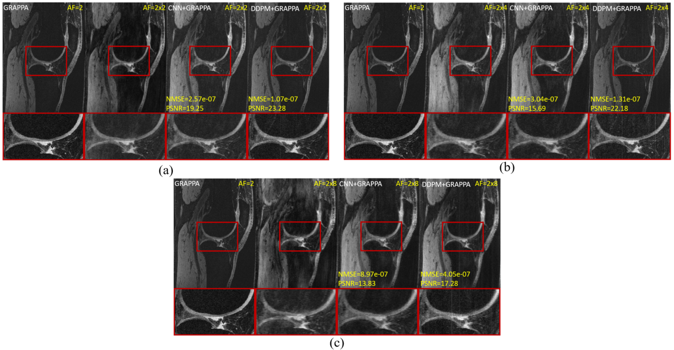
A total of five in-vivo knee images were scanned on a 3T Siemens scanner with a 15-channel coil. A 3D DESS sequence was scanned with TE=6.02ms, TR=17.55ms, and flip angle=20°. FOV=140 mm, slice thickness=0.7mm, matrix size=384x307x160 with GRAPPA factor of 2 ($$$\psi=2$$$). Among these data, Four images from a single channel but different knees (phase and slice-encoding directions, 384x4 images) were used for training and the rest images were used for testing the network. The GRAPPA data was retrospectively undersampled with 2D random undersampling patterns ($$$\omega=2,4,8$$$) to simulate combined acceleration factors of 2(GRAPPA)×2(DDPM), 2×4, and 2×8.
For comparison, we combined CNN⁶ with GRAPPA and show reconstructed images in Fig.2. The DDPM+GRAPPA is superior to CNN+GRAPPA in terms of reconstruction quality due to DDPM generating samples by a reverse diffusion process, which maps a simple Gaussian distribution, to the complex data distribution. This mapping is often complex in CNN. The corresponding PSNRS and NMSE shown on the bottom left of each image also indicated the DDPM is better.

Conclusion

In this abstract, we studied a combination of DDPM and GRAPPA for highly accelerated 3D knee imaging. Experimental results show that the proposed method can further accelerate the acquisition time by a factor of 8 on top of the GRAPPA factor of 2. More data sets will be used for evaluating tissue quantification accuracy in future studies.

Acknowledgements

This work is supported by NIH/NIAMS R01 AR077452