4030
Simulating BOLD fMRI transverse relaxation at 3 T: How accurate is the infinite cylinder model of blood vessels?1Department of Physics, Carleton University, Ottawa, ON, Canada, 2University of Ottawa Institute of Mental Health Research, Ottawa, ON, Canada, 3Rotman Research Institute, Baycrest Health Sciences, North York, ON, Canada, 4Athinoula A. Martinos Center for Biomedical Imaging, Massachusetts General Hospital, Charlestown, MA, United States, 5Department of Radiology, Harvard Medical School, Boston, MA, United States, 6Harvard-MIT Division of Health Sciences and Technology, Massachusetts Institute of Technology, Cambridge, MA, United States, 7Department of Medical Biophysics, University of Toronto, Toronto, ON, Canada
Synopsis
Keywords: Simulations, fMRI
Simulations of the BOLD signal have provided invaluable insights into the biophysical underpinnings of BOLD contrast. Typically, infinite cylinders are used to represent the vasculature, although, in reality the vasculature is much more complex. In this study, we compared several biophysical modelling techniques for simulating the BOLD effect, including using Vascular Anatomical Networks (VANs) to model the capillary bed with realistic geometry. We found the majority of the different simulation approaches produced relatively consistent results with each other. The VAN simulations were consistent with the infinite cylinders, suggesting that infinite cylinders are a reasonable approximation to more realistic vascular models.Introduction
Simulations of the BOLD signal have provided invaluable insights into the biophysical underpinnings of BOLD contrast1–5, and have in part shaped the development of techniques such as calibrated BOLD, qBOLD6, and vascular fingerprinting7. Since the development of BOLD fMRI, three-dimensional (3D) Monte Carlo simulations using infinite cylinders to represent blood vessels have been the gold standard in terms of simulation accuracy and flexibility. However, ever since the preliminary studies on the BOLD effect and increasingly so today, various adaptations of the simulation techniques have been implemented to accelerate the simulations or to make them compatible with geometries besides infinite cylinders. Ultimately, the goal is to model realistic vascular anatomy; however, until the recent development of vascular anatomical networks (VANs)5,8, it has been challenging to represent realistic vasculature in simulations accurately. In this study, we compared several major biophysical modelling techniques for simulating the BOLD effect, including VANs to model the capillary bed.Theory
“Gold Standard” SimulationOur gold standard reference simulation was a 3D voxel populated with randomly oriented infinite cylinders. For a magnetic susceptibility offset, Δχ, of blood relative to tissue, the intravascular (IV) and extravascular (EV) B0 perturbations are given in Fig. 1. To calculate the signal from the voxel, the Monte Carlo (MC) method was used: the positions of N spin bearing particles were randomly assigned, then their diffusion was modelled by randomly drawing displacements independently along x, y, and z from a Gaussian distribution with $$$\sigma=2D\delta t$$$, where D is the diffusion coefficient and δt is the time increment. This simulation is denoted by the string “3D-ANA-MC” for 3D voxel, analytical B0 calculations, MC-based diffusion.
2D Simulations
Two-dimensional (2D) simulations were first introduced as a time-saving alternative9, with infinite vessels oriented along z, perpendicular to the plane. We implemented 2D simulations that calculated the B0 offsets in two ways (Fig. 1): the B0 direction was randomly assigned to each vessel (2D-ANA-MC)10,11; or, B0 offsets were given as the average offset from three orthogonal B0 directions (B0 along x, y, z) (2D-ANA-MC-3B0)12.
FFT-based B0 Offsets
ΔB0 can be obtained by convolving the Δχ distribution with a point-source dipole field13,14. This convolution was performed in the frequency domain using the fast Fourier transform (FFT), returning ΔB0 on a discrete grid. Cyclic convolution was used to model the effects of surrounding vasculature at the same volume fraction. Using randomly oriented cylinders that span the voxel, this simulation is denoted “3D-FFT-MC”.
As an intermediate step between the gold standard and FFT-based simulations, we performed simulations where spin position was tracked in continuous space, however, ΔB0 was calculated analytically on a fixed grid. This is denoted “3D-ANA-MC-GRID”.
Vascular Anatomical Networks
We synthesized a set of realistic vascular anatomical networks (VANs) that feature uniform vascular radii while exhibiting realistic vascular features such as tortuosity and branching. The capillary bed consists of tortuous vessels made from smoothly connected, finite cylinders without overlap. The segment statistics and branching patterns were previously validated15,16. The FFT-ΔB0 calculation was necessarily used and the simulations were denoted “3D-VAN-FFT-MC”.
Methods
All simulations were implemented in Python v.3.10. We simulatedran a spin-echo sequence with the following settings: δt = 0.2 ms, D = 1 um2/ms, echo-time = 70 ms, B0 = 3T, Δχ = 4π×3.3×10–8 (65% oxygenation and 35% hematocrit). No intrinsic T2 decay was included. 10 random voxels were populated with 1-μm radius vessels to a blood-volume fraction of 2%. For MC simulations, 4×10⁴ spin histories were calculated per voxel.Two sets of comparisons were run independently for the IV, EV and total (EV+IV) signals. The signals, averaged over all 10 voxels, were compared to the average 3D-ANA-MC (gold standard) simulations using normalized root-mean-square-error (NRMSE). Next, “Boxerman” plots of the apparent relaxation rates were calculated as a function of radius as:$$ \Delta R_2^{(\prime)}=-\frac{1}{TE}\text{log}\left[\frac{S(TE)}{S(0)}\right].$$Using TE=30 ms for $$$\Delta R_2^{\prime}$$$ and TE=70 ms for $$$\Delta R_2$$$.
Results
The NRMSE of all simulation techniques relative to 3D-ANA-MC are plotted in Fig. 2. The Boxerman-style plots comparing all 3D simulations are given in Fig. 3, and all 2D simulations in Fig. 4. The 3D-ANA-MC-GRID, 2D-ANA-MC, 2D-ANA-DD simulations were most consistent with the reference (3D-ANA-MC). The 2D-ANA-MC-3B0 simulations were the least consistent and generally biased. For all, the IV signal was the most inconsistent.Discussion and Conclusions
Most of our wide range of simulation techniques were in good agreement with the reference (3D-ANA-MC) with NRMSE ~0.01–1% for EV signals. This suggests that any of these methods can be reliably adopted based on one’s requirements, except for the 3B0 method, which was the least accurate. Of note, we presented a comparison of simulations from VANs and infinite cylinders for the first time. The EV signal behaviour is remarkably similar, whereas the VAN IV signal diverges at small diameters. Since the FFT simulations using infinite cylinders were consistent with the reference, we think this difference is driven by differences in the morphology rather than in the simulation approach; however, this should be investigated further. To summarize, we found that realistic non-cylindrical vascular geometry is well approximated by random infinite cylinders.Acknowledgements
This work was supported in part by the NSERC (RGPIN-2022-04886), CIHR (MFE-164755 and FDN-148398), the NIH NIBIB (grants P41-EB030006 and R01-EB032746), the NIH NINDS (grant R01-NS128843), and by the BRAIN Initiative (NIH NIMH grants R01-MH111419, R01-MH111438, F32-MH125599, and U19-NS123717).References
1. Ogawa S, Menon RS, Tank DW, et al. Functional brain mapping by blood oxygenation level-dependent contrast magnetic resonance imaging. A comparison of signal characteristics with a biophysical model. Biophys J 1993;64:803–812 doi: 10.1016/S0006-3495(93)81441-3.
2. Boxerman JL, Hamberg LM, Rosen BR, Weisskoff RM. MR Contrast Due to Intravascular Magnetic-Susceptibility Perturbations. Magn Reson Med 1995;34:555–566.
3. Martindale J, Kennerley AJ, Johnston D, Zheng Y, Mayhew JE. Theory and generalization of Monte Carlo models of the BOLD signal source. Magn Reson Med 2008;59:607–618 doi: 10.1002/mrm.21512.
4. Uludag K, Muller-Bierl B, Ugurbil K. An integrative model for neuronal activity-induced signal changes for gradient and spin echo functional imaging. Neuroimage 2009;48:150–165 doi: 10.1016/j.neuroimage.2009.05.051.
5. Gagnon L, Sakadžić S, Lesage F, et al. Quantifying the microvascular origin of bold-fMRI from first principles with two-photon microscopy and an oxygen-sensitive nanoprobe. J. Neurosci. 2015;35:3663–3675 doi: 10.1523/JNEUROSCI.3555-14.2015.
6. He X, Yablonskiy DA. Quantitative BOLD: mapping of human cerebral deoxygenated blood volume and oxygen extraction fraction: default state. Magn Reson Med 2007;57:115–126 doi: 10.1002/mrm.21108.
7. Christen T, Pannetier NA, Ni W, et al. MR vascular fingerprinting: A new approach to compute cerebral blood volume, mean vessel radius, and oxygenation maps in the human brain. Neuroimage 2013 doi: 10.1016/j.neuroimage.2013.11.052.
8. Hartung G, Vesel C, Morley R, et al. Simulations of blood as a suspension predicts a depth dependent hematocrit in the circulation throughout the cerebral cortex. PLoS Comput. Biol. 2018;14 doi: 10.1371/journal.pcbi.1006549.
9. Bandettini PA, Wong EC. Effects of Biophysical and Physiological-Parameters on Brain Activation-Induced R(2)Asterisk and R(2) Changes - Simulations Using a Deterministic Diffusion-Model. Int. J. Imaging Syst. Technol. 1995;6:133–152 doi: Doi 10.1002/Ima.1850060203.
10. Miller KL, Jezzard P. Modeling SSFP functional MRI contrast in the brain. Magn Reson Med 2008;60:661–673 doi: 10.1002/mrm.21690.
11. Berman AJL, Mazerolle EL, MacDonald ME, Blockley NP, Luh W-M, Pike GB. Gas-free calibrated fMRI with a correction for vessel-size sensitivity. Neuroimage 2018;169:176–188 doi: 10.1016/j.neuroimage.2017.12.047.
12. Pannetier NA, Debacker CS, Mauconduit F, Christen T, Barbier EL. A simulation tool for dynamic contrast enhanced MRI. PLoS One 2013;8:e57636 doi: 10.1371/journal.pone.0057636.
13. Salomir R, De Senneville BD, Moonen CTW. A fast calculation method for magnetic field inhomogeneity due to an arbitrary distribution of bulk susceptibility. Concepts Magn. Reson. Part B-Magnetic Reson. Eng. 2003;19B:26–34 doi: Doi 10.1002/Cmr.B.10083.
14. Marques JP, Bowtell R. Application of a fourier-based method for rapid calculation of field inhomogeneity due to spatial variation of magnetic susceptibility. Concepts Magn. Reson. Part B-Magnetic Reson. Eng. 2005;25B:65–78 doi: Doi 10.1002/Cmr.B.20034.
15. Linninger A, Hartung G, Badr S, Morley R. Mathematical synthesis of the cortical circulation for the whole mouse brain-part I. theory and image integration. Comput. Biol. Med. 2019;110:265–275 doi: 10.1016/j.compbiomed.2019.05.004.
16. Hartung G, Badr S, Moeini M, et al. Voxelized simulation of cerebral oxygen perfusion elucidates hypoxia in aged mouse cortex. PLoS Comput. Biol. 2021;17:1–28 doi: 10.1371/JOURNAL.PCBI.1008584.
Figures
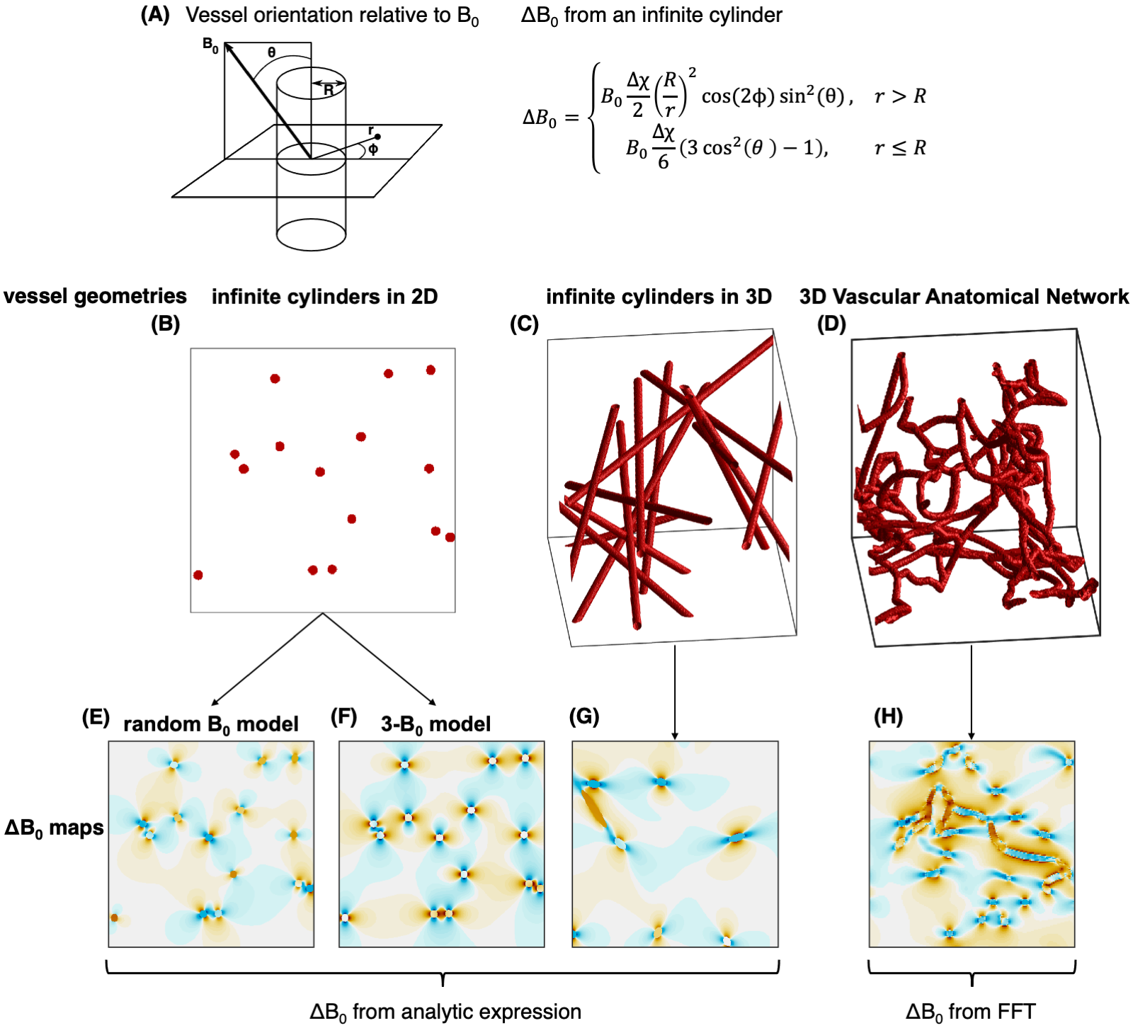
Fig 1: (A) Analytical field offset calculation for an infinite cylinder. (B–D) the different vessel geometries are examined in order of increasing complexity. (B) Infinite cylinders passing through a 2D plane. (C) Randomly oriented infinite cylinders in 3D. (D) A 3D VAN with finite, branching cylinders. (E–H) Corresponding field offsets through the networks. (E) and (F) are from the 2D geometry using two different models for calculating the field offsets. (G) uses the infinite cylinder analytic expression, and (H) uses the FFT offset calculation.
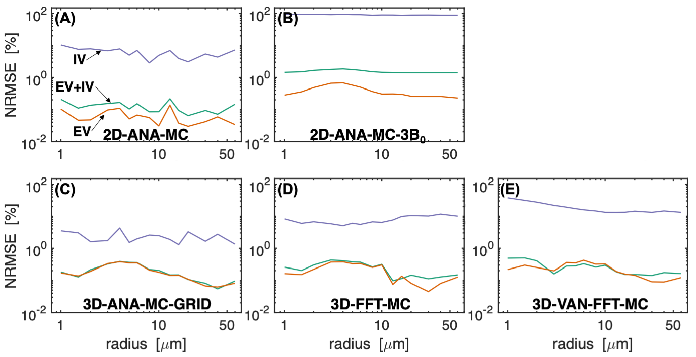
Fig 2: Normalized RMS error (in percent) vs. vessel radius for each simulation type. Comparisons are relative to the 3D random infinite cylinder Monte Carlo simulations (3D-ANA-MC). Comparisons were performed separately for the total (EV+IV) signal (green line), EV (orange), and IV (purple). Comparisons the 2D geometries are in the top row (A,B) and comparisons to the 3D geometries are in the bottom row (C–E), with the VAN results last (E).
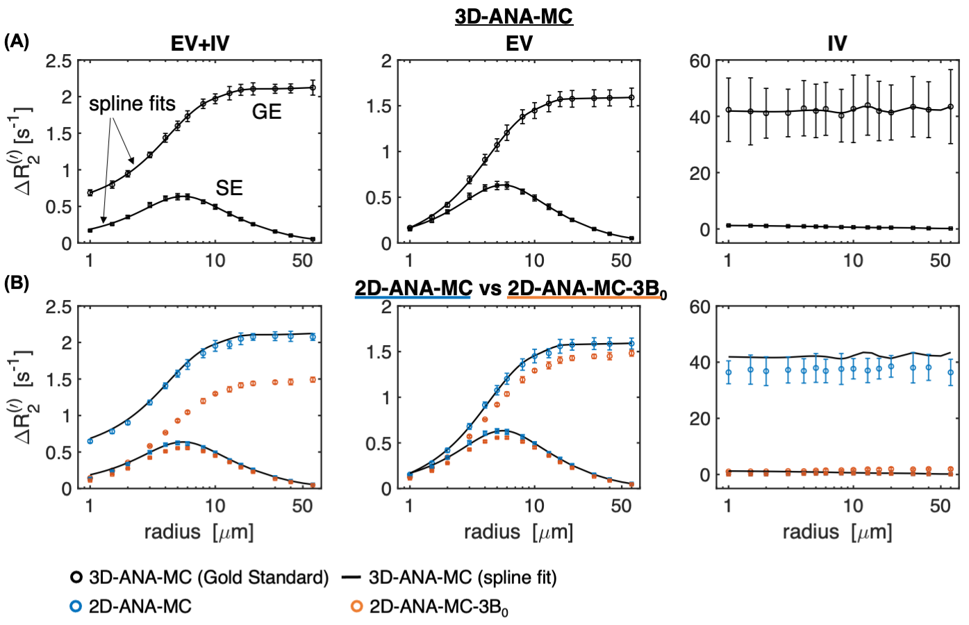
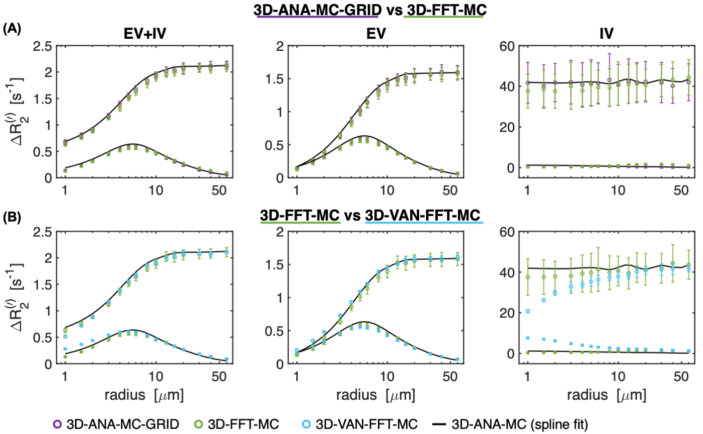
Fig 4: Boxerman plots showing the GE and spin-echo SE relaxation rates as a function of vessel radius for all 3D geometries. The black curve is the same spline fit from the gold standard in Fig 3A. (A) The effect of gridding the analytical field offsets (3D-ANA-MC-GRID) is compared to calculating ΔB0 using the FFT method on infinite cylinders (3D-FFT-MC). Both simulations are in close agreement. (B) The VAN simulations are compared against infinite cylinder simulations where each used the FFT method. The simulations agree well but there is some divergence for the IV signal at small radii.