4028
BOLDSwimSuite: A Python-based tool suite for numerical simulations of transverse relaxation in the presence of diverse field perturbers1Rotman Research Institute, North York, ON, Canada, 2Department of Physics, Carleton University, Ottawa, ON, Canada, 3University of Ottawa Institute of Mental Health Research, Ottawa, ON, Canada, 4Department of Medical Biophysics, University of Toronto, Toronto, ON, Canada
Synopsis
Keywords: Simulations, Software Tools
Numerical simulations are valuable tools for understanding the transverse relaxation process, but their use is impeded by computational complexities and a lack of standard in simulation pipelines. We present a new software suite (named BOLDSwimSuite) to address these challenges, making numerical simulations accessible to a wider community of researchers. Among its many features, this toolbox is able to accommodate arbitrary magnetic-field perturbers as well as simulate different MRI sequences. This toolbox is useful for investigating BOLD fMRI contrast and MR vascular fingerprinting among other applications.Introduction
Numerical simulations of transverse relaxation (R2’) are useful for understanding and predicting BOLD fMRI contrast1,2, for determining quantitative fMRI metrics of brain physiology using qBOLD, vascular fingerprinting3–5, or dynamic-susceptibility contrast MRI, for R2-based iron mapping6, and even for understanding diffusion-weighted MRI signals7. However, there are currently a wide variety of approaches to such numerical simulations8–11, which may contribute to inconsistencies in research findings in manners that are yet unknown. To support open science, we see tremendous value in creating a suite of tools for numerical simulations that provide researchers with a publicly available, user-friendly and customizable simulation experience that promotes reproducible research. In this work, we introduce such a software suite, named BOLDSwimSuite.Methods
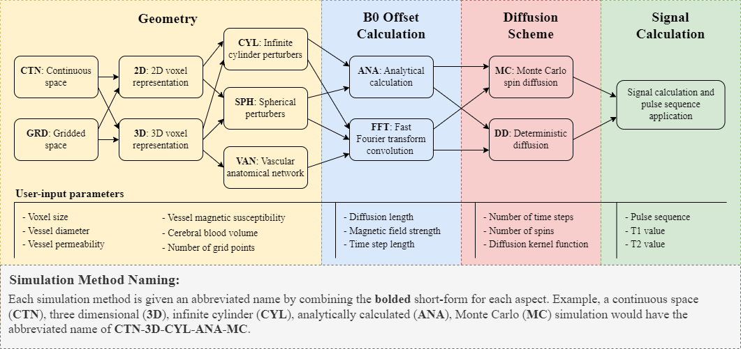
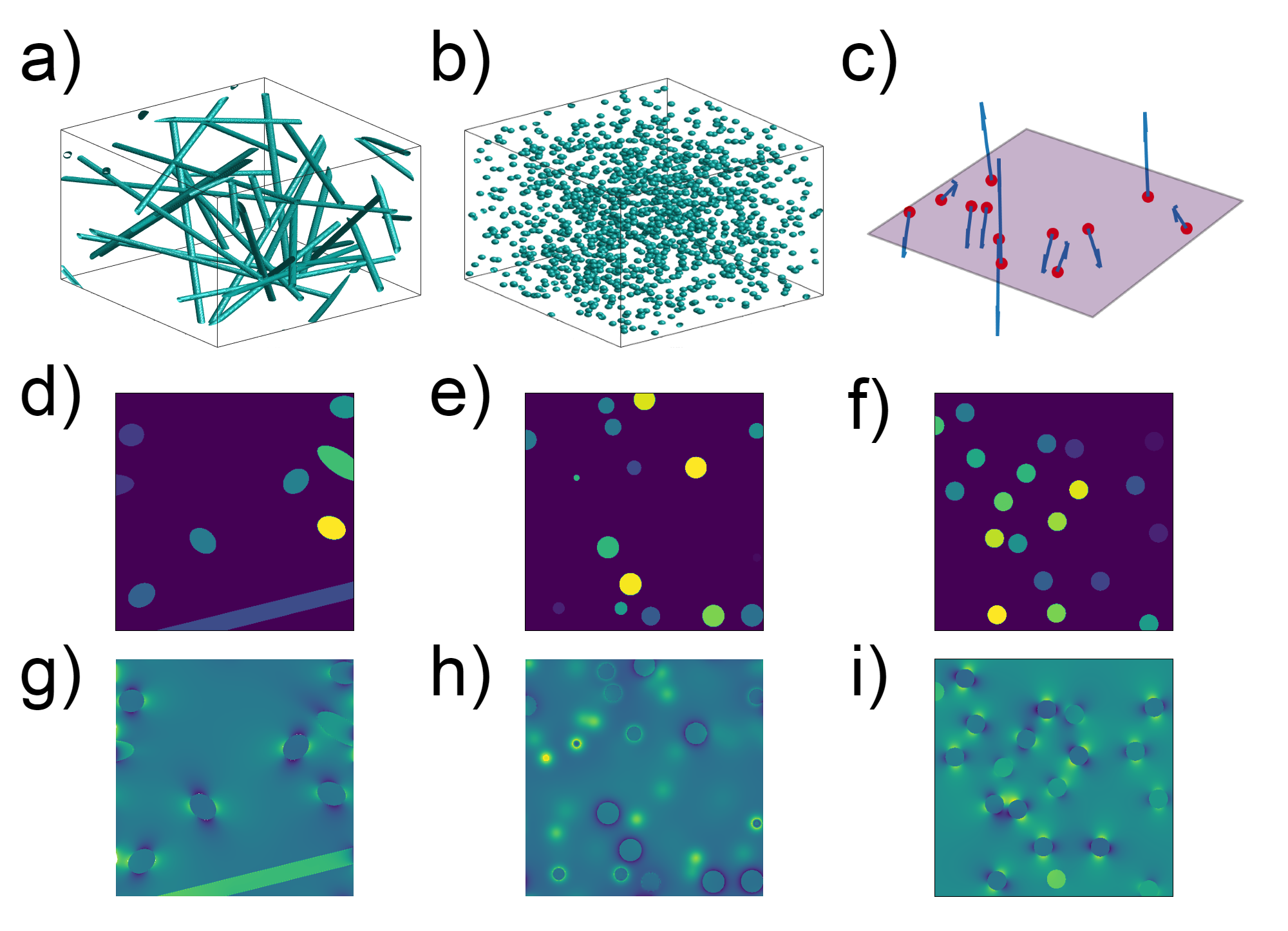
BOLDSwimSuite was implemented in Python 3.10. Its workflow consists of four main components: (1) perturber-geometry definition, (2) B0-offset calculation, (3) diffusion scheme and (4) signal calculation (Figure 1). They are connected to produce a pipeline. The user-input parameters are shown for each component, although not all are necessary for all simulation methods (e.g. continuous space simulations do not require a grid size as they do not operate on a grid). Due to the large number of method combinations that can be produced by this tool, a simple naming scheme has been devised to create short but comprehensive names. Refer to Figure 1 to understand these names. Under “Geometry”, the first choice is between continuous (CTN) and discrete (GRD) space options3,12. Continuous-space simulations use infinitesimal sub-voxel sizes (within floating point accuracy) but require an analytical B0-offset calculation (ANA). Discrete-space simulations operate on highly discretized spatial coordinates (“gridded”) and can be used with either analytical (ANA) or fast-Fourier convolution (FFT) based B0 calculation13. The next choice is between 2D and 3D simulations. Finally, the perturbers can be infinite cylinders, spheres or arbitrary configurations such as vascular-anatomical networks (VANs) (Figure 2).Next, in the “B0 offset calculation” component, available options include ANA or FFT, as mentioned earlier (see Figure 2(g)-(i) for samples). The ANA option is limited to known perturber models such as infinite cylinders and spheres, whereas the FFT option, which requires a gridded space, can also accommodate arbitrary perturber geometries such as VANs.
Diffusion of spins alters the observed R2 especially in the presence of microscopic field perturbers, and available diffusion schemes include Monte Carlo (MC) and deterministic (DET). The former makes use of randomly positioned spins that are randomly moved in the simulated voxel and individually accumulate phase offset, and is considered the de-facto gold-standard. The latter choice uses convolution with a deterministic-diffusion kernel to approximate the diffusion process, and is implemented on a gridded space.
The final step is “Signal Calculation”, which integrates the dephasing spins or samples with the user-defined pulse sequence to produce the output signal time course. The toolbox provides the external signal (EV), internal signal (IV) and the total signal (IV+EV).
Results
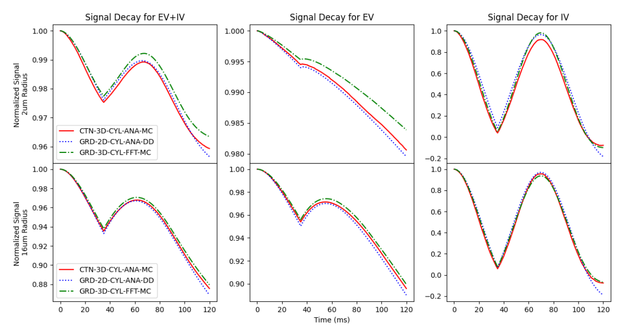
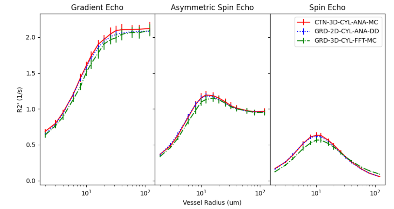
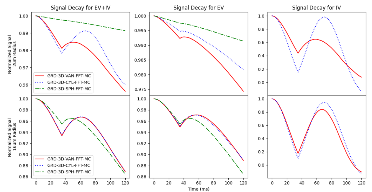
A few examples of the wide array of possible outputs from BOLDSwimSuite are shown in Figures 3-5 to demonstrate the toolbox’s capabilities. Figure 3 shows the generated transverse signal decays for three possible simulation pipelines on the same perturber geometry (infinite cylinders). Figure 4 shows the cylinder-size dependence of R2’ corresponding to these simulation pipelines, resulting from a gradient echo (GE), spin echo (SE) and asymmetric spin echo (ASE) pulse sequences. R2’ is derived by sampling the signal decay at different timepoints. Figure 5 shows the R2’ signal decay for different perturber geometries (i.e. infinite cylinder, spheres or VAN), based on the 3D FFT-B0 MC-diffusion pipeline, for perturber radii of 2um and 12um. Cylindrical and spherical perturbers of the same radii diverge substantially in their R2’ decay curves, with the former more closely resembling the results for a VAN perturber. All Monte Carlo results are based on the use of 40,000 spins.Discussion & Conclusions
In the current implementation of BOLDSwimSuite, infinite cylinders have analytically defined B0 offsets for both the IV and EV compartments (i.e. intra- and extravascular), while only the external B0 offset is defined for spheres. Other perturbers from the VAN (such as a white-matter voxel) can also be input to the simulation. Additionally, while the current simulations focus on voxels with uniform perturber sizes, more realistic distributions of different perturber sizes can also be specified. Moreover, 2D simulations present lower computational requirements at the cost of reduced modeling accuracy and flexibility in perturber morphometry. Furthermore, Monte Carlo diffusion is generally more flexible but results in greater signal variability especially when used with lower spin counts. On the other hand, deterministic diffusion is less flexible (e.g. requires a gridded space) and is more computationally demanding (due to the convolution step), but produces little to no variability in the output signal. Lastly, when completed, we plan to make the toolbox available upon request.Acknowledgements
This work was supported by the Canadian Institutes of Health Research and the Natural Sciences and Engineer Research Council of Canada as well as CIHR grant FDN-148398, CIHR grant MFE-16475 and NSERC grant RGPIN-2022-04886.References
1. Uludağ K, Müller-Bierl B, Uğurbil K. An integrative model for neuronal activity-induced signal changes for gradient and spin echo functional imaging. Neuroimage. 2009;48:150–65.
2. Boxerman JL, Hamberg LM, Rosen BR, Weisskoff RM. MR contrast due to intravascular magnetic susceptibility perturbations. Magn Reson Med. 1995;34(4):555–66.
3. Christen T, Pannetier NA, Ni WW, Qiu D, Moseley ME, Schuff N, et al. MR vascular fingerprinting: A new approach to compute cerebral blood volume, mean vessel radius, and oxygenation maps in the human brain. Neuroimage. 2014 Apr 1;89:262–70.
4. Stone AJ, Holland NC, Berman AJL, Blockley NP. Simulations of the effect of diffusion on asymmetric spin echo based quantitative BOLD: An investigation of the origin of deoxygenated blood volume overestimation [Internet]. Available from: http://dx.doi.org/10.1101/570697
5. Berman AJL, Mazerolle EL, MacDonald ME, Blockley NP, Luh WM, Pike GB. Gas-free calibrated fMRI with a correction for vessel-size sensitivity. Neuroimage. 2018 Apr 1;169:176–88.
6. Schenck JF. Imaging of brain iron by magnetic resonance: T2 relaxation at different field strengths. J Neurol Sci. 1995 Dec;134 Suppl:10–8.
7. Fieremans E, Lee HH. Physical and numerical phantoms for the validation of brain microstructural MRI: A cookbook. Neuroimage. 2018 Nov 15;182:39–61.
8. Berman AJL, Pike GB. Transverse signal decay under the weak field approximation: Theory and validation. Magn Reson Med. 2018 Jul;80(1):341–50.
9. Martindale J, Kennerley AJ, Johnston D, Zheng Y, Mayhew JE. Theory and generalization of Monte Carlo models of the BOLD signal source. Magn Reson Med. 2008 Mar;59(3):607–18.
10. Klassen LM, Menon RS. NMR simulation analysis of statistical effects on quantifying cerebrovascular parameters. Biophys J. 2007 Feb 1;92(3):1014–21.
11. Pannetier NA, Sohlin M, Christen T. Numerical modeling of susceptibility‐related MR signal dephasing with vessel size measurement: Phantom validation at 3T. Magnetic resonance [Internet]. 2014; Available from: https://onlinelibrary.wiley.com/doi/abs/10.1002/mrm.24968
12. Boxerman JL, Bandettini PA, Kwong KK, Baker JR, Davis TL, Rosen BR, et al. The intravascular contribution to fMRI signal change: Monte Carlo modeling and diffusion-weighted studies in vivo. Magn Reson Med. 1995 Jul;34(1):4–10.
13. Deville G, Bernier M, Delrieux JM. NMR multiple echoes observed in solidHe3 [Internet]. Vol. 19, Physical Review B. 1979. p. 5666–88. Available from: http://dx.doi.org/10.1103/physrevb.19.5666
Figures