Synopsis

Keywords: Machine Learning/Artificial Intelligence, Diffusion/other diffusion imaging techniques

Advanced diffusion weighted self-navigated multi-shot MRI can run at high scan efficiencies resulting in good image quality. However, the model-based image reconstruction is rather time consuming. Deep learning-based reconstruction approaches could function as a faster alternative. Tailored network architectures with appropriately set physical model constraints can help to shorten reconstruction times, resulting in good image quality with reduced noise propagation.

Introduction

Single-shot EPI is one of the standard protocols for diffusion-weighted imaging (DWI) in clinical practice¹. However, the relatively long readout time of single-shot acquisitions may result in signal loss, image blur, and large geometric distortions. Consequently, multi-shot EPI (msh-EPI) has become an increasingly preferred method for DWI to produce high-resolution images with less geometric distortion^2,3. However, an inherent challenge for msh-EPI-based DWI is the occurrence of shot-to-shot phase errors induced by physiological motion in presence of the strong diffusion-sensitizing gradients. Many studies have proposed to use either additionally measured navigators² or self-navigation^4,5 corrections to deal with such phase errors. However, these methods may either prolong scan-times or reconstruction times. In this work, a neural network with two U-net architectures was trained to reconstruct a shot-specific phase map for each shot and one joint magnitude image. Those were merged, including physical model constraints, in the joint loss calculation of the two U-nets^6,7. This approach not only realizes fast image reconstruction, but also benefits from image denoising due to the choice of training data and the nature of convolutional neural networks (CNNs). In this work, the training pairs for DWI were simulated using T2w leg images with extra noise added to mimic the lower SNR in diffusion measurements.

Methods

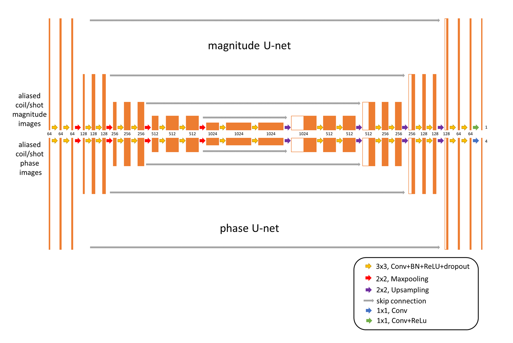
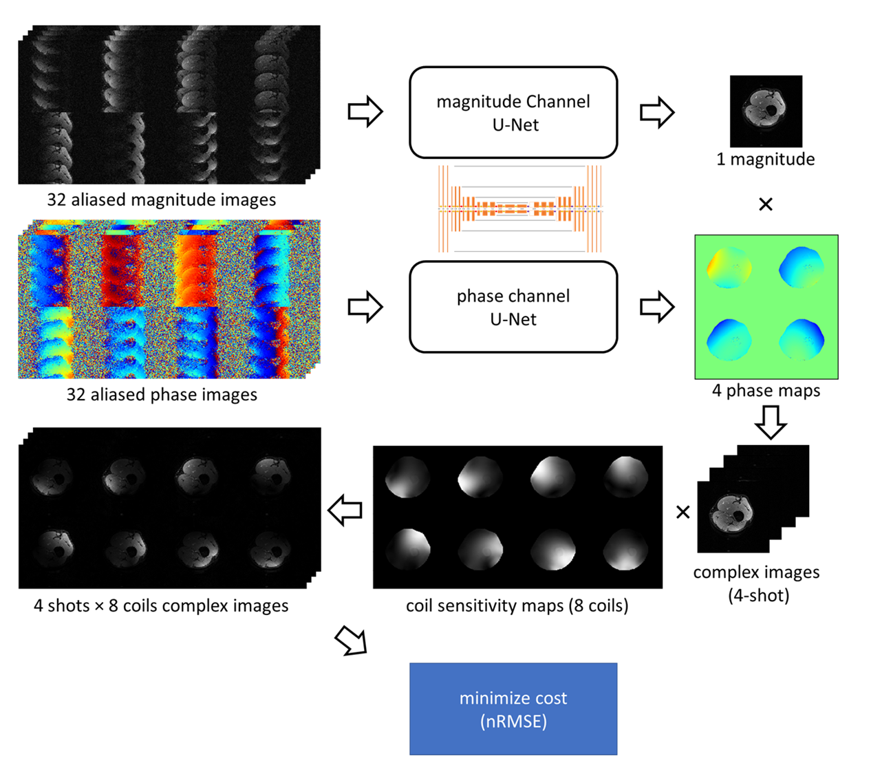
Inspired by many self-navigation approaches in DWI, in this work a joint image constraint was set up by assuming all different shots share one underlying magnitude representation in combination with different, shot-specific phases. Two separate U-net-like CNNs for magnitude and phase components were trained together using a combined loss function (see Fig.1). The outputs of the two individual CNNs were concatenated to calculate a joint loss. The signal model of the msh-EPI-based DWI can be expressed as:$$S_{i,l}={K_i}{F}{C_l}{e^{j\phi_i}}I$$where $$$S_{i,l}$$$ is the k-space data of the $$$i$$$-th shot and $$$l$$$-th coil, $$$K_i$$$ is the sampling operator, $$$F$$$ is the Fourier transform operator, $$$C_l$$$ is the coil sensitivity, and $$$\phi_i$$$ and $$$I$$$ are the shot-specific phase maps and the joint magnitude that need to be estimated. The task of the network is to minimize:
$$\operatorname{loss}\left(I,\phi_i\right)=\sum_i \sum_l\left\|f_m(X)\cdot{e^{j{f_p(P)_i}}}\cdot{C_l}-M_{i,l}\right\|_2^2$$where $$$f_m(X)=\mathrm{I}$$$ is the joint magnitude predicted by the first “magnitude” U-net, and $$$f_p(P)_i=\phi_i$$$ is the i-th shot’s phase map predicted by the second “phase” U-net The aliased magnitude images $$$X$$$ and phase images $$$P$$$ are the separate inputs of the two U-nets, and are calculated by taking the magnitude and phase from the inverse Fourier transform of each shot $$$i$$$ and coil $$$l$$$ of zero-filled k-space data $$$S_{i,l}$$$. $$$M_{i,l}$$$ denotes the ground truth image for the loss calculation, which can be calculated via $$$M_{i,l}=C_l{e^{j\phi_i}}I$$$. The architecture of the network is shown in Fig. 1.
The training data were generated from b=0 s/mm² leg images (from 18 volunteers) measured in the knee/lower leg (3T, Philips, Best, The Netherlands). The scan parameters can be found in Table 1. In this work, 4-shot and 8-coils diffusion data were simulated for training. To generate training inputs, each corresponding series of the 4-shot images (and 8 coils) were undersampled with R=4 according to the 4-shot msh-EPI trajectory. Data augmentation was performed by randomly applying in-plane rotation, flipping, and resizing. Varying shot-specific phases were simulated based on a second-order random Gaussian profile with spatial variation between ± π. To simulate low SNR at higher b-values, random complex Gaussian noise was added to the training input for SNR levels ranging between 8 to 26. Two different models were trained with/without synthetic noise added to the target sets, to obtain two networks with/without strong denoising ability. In total, 1120 different 4-shots DW synthetic training pairs were generated, which are divided into 32 aliased magnitude/phase images as inputs for each U-net, and 32 complex fully k-space data as target sets. The loss function calculation is illustrated in Fig. 2. The training was run for 400 epochs with a batch size of 5, using the Adam optimizer with a learning rate of 0.0001.
Test data were measured using a fat-suppressed DW 4-shot msh-EPI sequence of 2 volunteers’ leg on the 3T scanner. The deep learning results were compared to model-based results using extra-navigated² and two self-navigated methods (POCS-ICE⁴, MUSSELS⁵).

Results

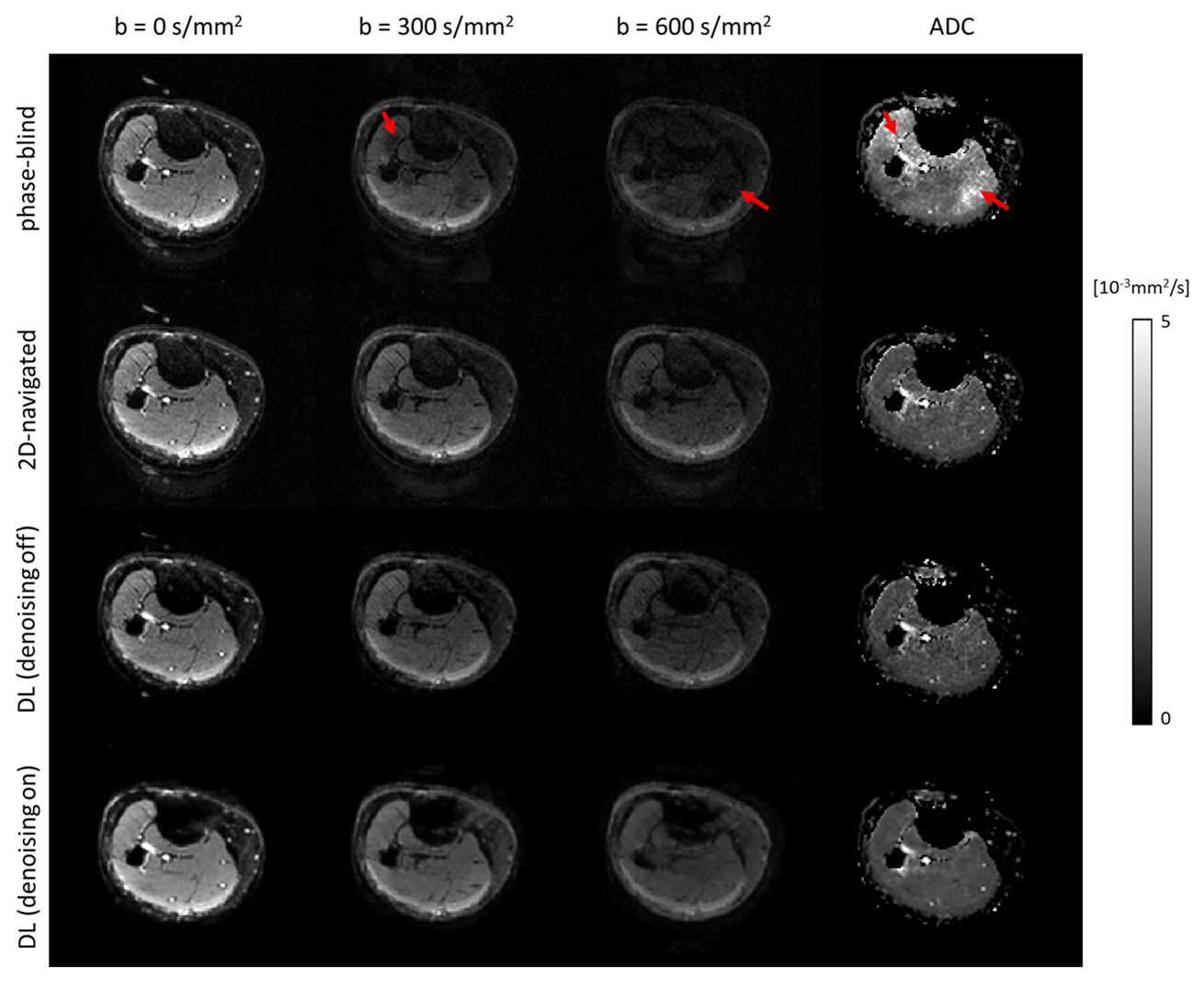
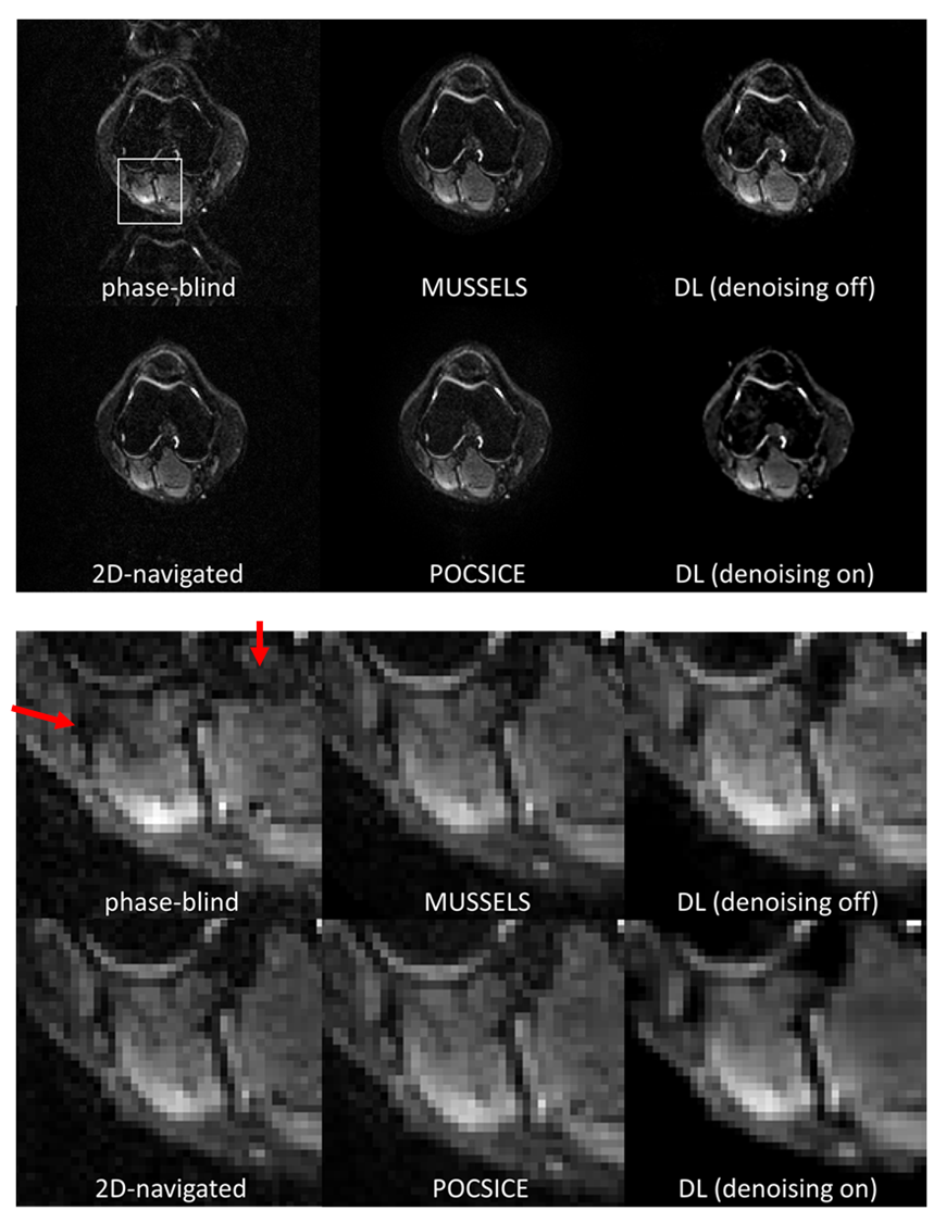
Fig. 3 shows the reconstructions and corresponding ADC maps of three b-values, qualitatively comparing no-navigation, extra-navigated, and deep learning reconstruction with denoising training on/off. Fig. 4 shows comparisons between different methods (2D-navigated²,MUSSELS⁴,POCS-ICE⁵). The network outperformed all the other methods in terms of reconstruction speed (see the caption of Fig.4.). The reduced noise floor is appreciated as well.

Discussion and conclusion

The fully deep learning-based multi-shot EPI reconstruction method proposed in this work demonstrates good preliminary results in the leg region based on simulated training pairs. This helps to accelerate the reconstruction of a joint full-k-space magnitude image compared to traditional model-based solutions. Specifically, the well-known challenge of correcting shot-to-shot phase variations in multi-shot acquisitions was addressed by using the "double" U-net architecture. In addition, due to the inherent properties of CNNs, denoising capability was also trained in the network. The next step will be to train on other anatomies (e.g. the brain), to test the robustness of the method and to prevent oversmoothing. More quantitative analysis is necessary and should be subject of future work.

Acknowledgements

The authors would like to acknowledge NWO-TTW (HTSM-17104).