Synopsis

Keywords: Data Analysis, Spectroscopy

It has been suggested that fitting dynamic MRS data in tandem (2D fitting) should be more precise than conventional 1D fitting, without impairing its accuracy. Functional MRS (fMRS) is a dynamic method used for detecting endogenous metabolic changes in the brain. In this work, we implemented a 2D spectral-temporal fitting framework for the synthetic fMRS data. Preliminary experiments confirm that 2D fitting improves precision approximately three-fold compared to the conventional 1D fitting in terms of fMRS data.

Introduction

Functional MRS (fMRS) is one of the dynamic MRS methods designed to detect endogenous metabolic changes in glutamate, GABA, and lactate in response to an external visual, motor, or cognitive manipulation [1]. Conventional analysis of fMRS is comprised of two stages: 1) Each spectrum is fitted with a linear combination of basis functions to obtain the amplitudes of each metabolite; 2) The time series for the amplitudes of each metabolite is analyzed separately, either directly or by fitting it to a dynamic model [2]-[5]. Recently, it has been suggested that fitting the dynamic data in tandem (2D fitting), which utilizes the temporal correlations inherent in the data, would provide more precise and accurate estimates of temporal constants [1], [6]-[8]. In this work, we quantified the expected gains to precision offered by 2D spectral-temporal fitting relative to conventional approaches, using synthetic fMRS data.

Theory and Methods

Spectral and Temporal Models
Assuming $$$s$$$ to be a spectral-temporal signal of fMRS data, $$$t$$$ is spectral time points and $$$T$$$ is temporal dynamic time points, the fMRS data can be modeled as: $$s(t,T) = {M_{global}}(t)\sum\limits_{j = 1}^J {T{D_j}(T){M_{local,j}}(t){f_j}(t) + B + N} (0,{\sigma ^2})$$
where $$$j$$$ denotes the number of metabolites, $$$TD$$$ is a temporal dynamic model, $$$M$$$ denotes the spectral model, $$$f$$$ is the basis from the transition table, $$$B$$$ denotes the B spline baseline, and $$$N$$$ is the white Gaussian noise.
1) Spectral Model
There are two spectral models in our work: the global spectral model for the sum of all metabolites and the local spectral model for each metabolite. They can be written as:
$${M_{local,j}}(t) = {A_j}{e^{2\pi i\frac{{{\phi _j}}}{{360}}}}{e^{2\pi i{\delta _j}t}}{e^{ - \frac{t}{{{d_j}}}}}$$
$${M_{global}}(t) = {A_{global}}{e^{2\pi i\frac{{{\phi _{global}}}}{{360}}}}{e^{2\pi i{\delta _{global}}t}}{e^{ - {d_{global}}{t^2}}}$$
where $$$A$$$ is the amplitude, $$$\phi $$$ denotes the phase in degree, $$$\delta $$$ denotes the shift, and $$$d$$$ indicates the damping factor.
2) Temporal Model
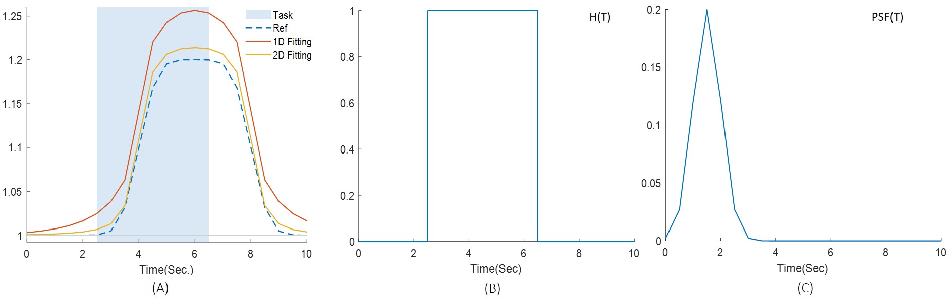
We assumed a boxcar external stimulus, $$$H(T)$$$, equal to unity for $$$T \in [{T_i},{T_f}]$$$ and zero elsewhere, and a linear response with a Gaussian point-spread-function, $$$PSF(T)$$$ with width $$$k$$$ and center at $$$\Delta $$$:
$$PSF(T) = \lambda {e^{( - \frac{{{{(T - \Delta )}^2}}}{{2{k^2}}})}}$$
$$\begin{array}{l}TD(T) = (1 + (PSF \otimes H))(T)\\{\rm{ }} = 1 + \frac{\lambda }{2}[{\rm{erf}}(\frac{{{T_f} - T + \Delta }}{{\sqrt 2 k}}) - {\rm{erf}}(\frac{{{T_i} - T + \Delta }}{{\sqrt 2 k}})]\end{array} $$
where $$$\lambda $$$ denotes the amplitude of the temporal response, and erf is the error function: $$${\rm{erf}}(x) = \frac{2}{{\sqrt \pi }}\int_0^x {{e^{ - {t^2}}}dt} $$$.
Synthetic Data Generation
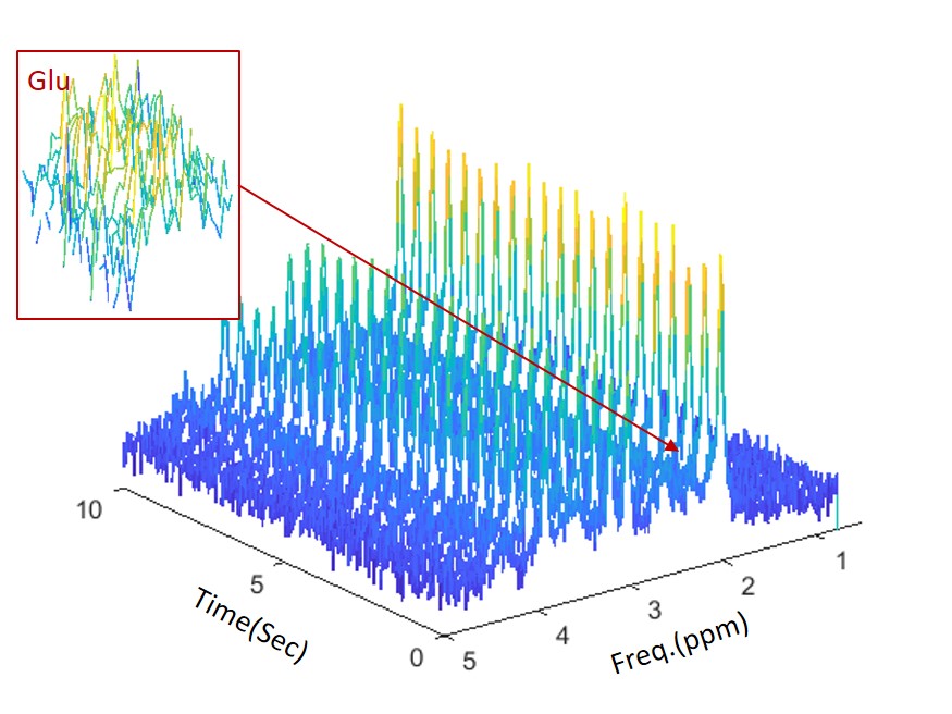
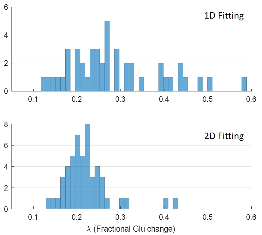
The experimental data used in this work is generated by in-house software VDI [9]. It contains 17 metabolites as per Ref. [10]. Only Glu is assumed to change over time, whereas other metabolites remain temporally static. For the Glu, the temporal parameters are set as: $$$\lambda = 0.2$$$, $$$k = 0.5$$$ seconds, $$$\Delta = 1.5$$$ seconds, $$${T_i} = 2.5$$$ seconds, and $$${T_f} = 6.5$$$ seconds. Spectra were generated for values of $$$T = 0, 0.5, ..., 10$$$ seconds. To evaluate the effect of noise, a set of white Gaussian noises (SNR = 15, 25, 35, 45, and 55) is added to the experimental data for fitting. The SNR was defined as the ratio between the maximum of the NAA singlet at 2.01 ppm and the standard deviation of the added noise. For each SNR, the precision (standard deviation) and bias (difference from ground truth) of each fitted parameter were calculated by repeating the simulation 50 times, each time with newly generated noise.

Results and Discussion

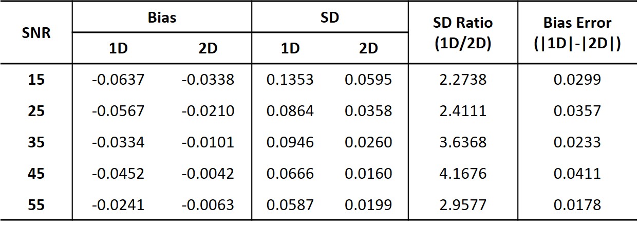
Figure 1 shows one example of the synthetic fMRS data with SNR = 25. To illustrate the accuracy and precision of the two methods, the temporal amplitude of Glu and the histogram of the estimated are plotted in Fig. 2(A) and 3, respectively. The external stimulus $$$H(T)$$$ and point-spread-function $$$PSF(T)$$$ used in this work are shown in Fig. 2(B) and (C). The fitting results under different noises are summarized in Table 1. It can be seen from Table 1 that 2D fitting improves the precision of the percent change of glutamate, $$$\lambda $$$, approximately three-fold, regardless of the SNR.

Conclusions

Our work demonstrates that simultaneous spectral-temporal fitting of synthetic fMRS data provides a substantial three-fold increase to the precision of fitted glutamate dynamics, without impairing its bias. This provides a strong impetus for transitioning to 2D model-based fitting approaches for in-vivo fMRS data.

Acknowledgements

This work is supported by the National Science Foundation of China (No. 62001290) and Sponsored by Shanghai Sailing Program (20YF1420900), and by the Israeli Science Foundation Personal Grant 416/20.