3905
Estimating noise figure of matching networks for low-input-impedance preamplifiers
Wenjun Wang1, Juan Diego Sánchez Heredia2, Vitaliy Zhurbenko1, and Jan Henrik Ardenkjær Larsen2
1National Space Institute, Technical University of Denmark, Kongens Lyngby, Denmark, 2Department of Health Technology, Technical University of Denmark, Kongens Lyngby, Denmark
1National Space Institute, Technical University of Denmark, Kongens Lyngby, Denmark, 2Department of Health Technology, Technical University of Denmark, Kongens Lyngby, Denmark
Synopsis
Keywords: RF Arrays & Systems, RF Arrays & Systems, matching
The noise figure of a matching network between a receive coil and a preamplifier with low input impedance can be estimated using relationship \(F\approx1+R_{11}/R_\mathrm{c}\). It is demonstrated how to use this relationship to choose optimal matching-decoupling network topology in terms of signal-to-noise ratio (SNR). The formula serves as an efficient tool to estimate noise figure of matching networks and is useful in low-field and high-coil-Q applications, where the noise of the matching network becomes comparable to coil noise.Introduction
Preamplifier decoupling is widely used in receive coil arrays to avoid detuning array elements unwantedly1. Design equations for ideal three-2 and four-element3 networks (or equivalent) have been reported. However, there is no explicit guideline for choosing circuits for better noise performance. Whereas resistive loss of networks can significantly degrade SNR at preamplifiers’ inputs, it largely relies on coil designers’ experience to discern the most SNR-degrading network component and to minimise SNR degradation. A diagram of an array element consisting of a coil, a preamplifier and a matching-decoupling network is illustrated in Figure 1. In the following sections, we show that the noise figure of the matching network can be estimated using $$F\approx1+\dfrac{R_{11}}{R_\mathrm{c}},\qquad(1)$$where $$$R_\mathrm{c}$$$ is the coil resistance and $$$R_{11}=\Re Z_{11}$$$ is the input impedance of the matching network $$$Z_\mathrm{i}$$$ when preamplifier A is disconnected. Equation (1) holds for typical low-input-impedance preamplifiers with $$$X_\mathrm{a}+X_\mathrm{o}=0$$$. It reveals that the SNR degradation is determined by the ratio between component loss defining $$$R_{11}$$$ and coil loss.Methods
To derive (1), $$$F$$$ is defined as the relation between the SNR before entering preamplifier A and the SNR on coil C: $$$\mathrm{SNR}_\mathrm{a}=\mathrm{SNR}_\mathrm{c}\times F^{-1}$$$. Unless otherwise noted, $$$X=\Im Z$$$, $$$R=\Re Z$$$. At 290 K, $$$F^{-1}=G_\mathrm{av}$$$.4 Figure 1 shows the expression of $$$G_\mathrm{av}$$$.5 From the relation between $$$Z_\mathrm{i}$$$ and $$$Z_\mathrm{o}$$$, we have $$-Z_{⌀}^{2}=\left(Z_\mathrm{i}-Z_{11}\right)\left(Z_{22}+Z_\mathrm{a}\right)=\left(Z_\mathrm{o}-Z_{22}\right)\left(Z_{11}+Z_\mathrm{c}\right).\qquad(2)$$ From (2) we solve $$Z_{22}=\dfrac{Z_\mathrm{a}\left(Z_{11}-Z_\mathrm{i}\right)+Z_\mathrm{o}\left( Z_\mathrm{c}+Z_{11}\right)}{Z_\mathrm{i}+Z_\mathrm{c}}\,.\qquad(3)$$ Therefore $$Z_\mathrm{o}-Z_{22}=\dfrac{\left(Z_\mathrm{i}-Z_{11}\right)\left( Z_\mathrm{o}+Z_\mathrm{a}\right)}{Z_\mathrm{i}+Z_\mathrm{c}}\,.\qquad(4)$$ For a lossless matching network, $$$\left.Z_{11}\right|_{\mathrm{lossless}}=-\mathrm{j}X_\mathrm{c}$$$ if $$$X_\mathrm{a} + X_\mathrm{o} = 0$$$ and the matching network is correctly tuned. $$$\left.\Im Z_\mathrm{i} \right|_{\mathrm{lossless}}=-X_\mathrm{c}$$$ yields the maximum preamplifier decoupling regardless of $$$X_\mathrm{a}+X_\mathrm{o}$$$.6 For low-loss matching networks, it is found in simulation and experiments that, if $$$X_\mathrm{a}+X_\mathrm{o}=0$$$, $$$\Im Z_{11}=-X_\mathrm{c}$$$ still holds well; $$$\Im Z_\mathrm{i}=-X_\mathrm{c}$$$ is also a close condition for maximum preamplifier decoupling. So assume $$$\Im Z_{11}=\Im Z_\mathrm{i}=-X_\mathrm{c}$$$; together with $$$X_\mathrm{a}+X_\mathrm{o}=0$$$, we infer that $$$\Im \left(Z_\mathrm{i}-Z_{11}\right) = 0$$$, $$$\Im \left(Z_\mathrm{o}+Z_\mathrm{a}\right)=0$$$, $$$\Im \left(Z_\mathrm{i}+Z_\mathrm{c}\right) = 0$$$. Then, using (4), $$$\Im \left(Z_\mathrm{o}-Z_{22} \right)=0$$$. We can then write $$$Z_\mathrm{o}-Z_{22}=R_\mathrm{o}-R_{22}$$$ and $$$Z_\mathrm{c}+Z_{11}=R_\mathrm{c}+R_{11}$$$. Substituting these into $$$G_{\mathrm{av}}$$$ in Figure 1, we get $$F=G_{\mathrm{av}}^{-1}=\dfrac{R_\mathrm{c}+R_{11}}{R_\mathrm{c}}\times\dfrac{R_\mathrm{o}}{R_\mathrm{o}-R_{22}}\,.\qquad(5)$$ Recall that $$$Z_{11}$$$ is defined by the input impedance at port 1 with port 2 disconnected, and $$$Z_{22}$$$ is defined by the input impedance at port 2 with port 1 disconnected7. Compared with $$$R_\mathrm{o}$$$—often 50 Ω and higher—$$$R_{22}$$$ of a low-loss matching network should be negligible. Neglecting $$$R_\mathrm{o}/\left( R_\mathrm{o}-R_{22}\right)$$$, we arrive at (1), thereby concluding the derivation.To demonstrate (1) and (5) at 32.13 MHz, the Larmor frequency of 13C at 3 T, oval mouse coils shown in Figure 2(a) are matched to WMA32C preamplifiers (WanTCom Inc., Chanhassen, MN, USA). The coil impedance $$$Z_\mathrm{c}=25.7~\mathrm{mΩ}+\mathrm{j}11.7~Ω$$$, output impedance $$$Z_\mathrm{o} =Z_\mathrm{n,opt}=52.04+\mathrm{j}0.07~Ω$$$ and preamplifier impedance $$$Z_\mathrm{a}=2.30-\mathrm{j}0.77~Ω$$$ for initial calculation. It follows that $$$X_\mathrm{a}+X_\mathrm{o}=-0.70~Ω$$$, close to 0. The three-2 and four-element3 matching networks are first calculated by corresponding formulae, and then realised by off-the-shelf components. Printed circuit boards (PCBs) are routed and simulated in Advanced Design System (Keysight Technologies, Santa Rosa, CA, USA). $$$F$$$ is extracted from simulations. PCBs are fabricated, and SNR values are measured on a bench top with an SMC100 signal generator (Rohde & Schwarz, Munich, Germany) and an Agilent E4440A spectrum analyser (Keysight Technologies, CA, USA). During simulation and experiments, initially capacitors and inductors are fine-tuned so that the maximum preamplifier decoupling is achieved for the mouse coil, and the output impedance is $$$Z_\mathrm{o}=Z_\mathrm{n,opt}=52~Ω$$$; then the peaks of SNR are tuned to 32.13 MHz. Capacitors are from PPI 1111C (Passive Plus Inc., Huntington, NY, USA). Inductors are from Coilcraft Inc. (Cary, IL, USA). Since our experiment is on a test bench, for simplicity, no active decoupling circuit is implemented.
Results
The measured coil current (preamplifier decoupling) and SNR are shown in Figure 3. The ratio of unloaded-to-loaded Q is shown in Figure 3. The simulated and estimated by (5) at 32.13 MHz are shown in Figure 4.Discussion
At 32.13 MHz, the measured SNR of the four-element network is higher than the SNR of the three-element network by 6.60 dB, which implies noise figure difference of 6.60 dB as both setups use the same preamplifier. Simulation predicts 7.33 dB SNR difference and 7.17 dB noise figure difference. Both are close to the measured 6.60 dB. As shown in Figure 4, $$$F$$$ estimated by (5) stands very close to simulated $$$F$$$, with errors below 0.29 dB, or 7.0%. It is also clear that the term $$$R_\mathrm{o}/\left(R_\mathrm{o}-R_{22}\right)$$$ in (5) is negligible. Thus in this case (5) can be simplified to (1). Equations (1) and (5) explain the difference between SNR (and $$$F$$$) using the four-element network in Figure 2(d) and the three-element network in Figure 2(c). The inductor in Figure 2(c) contributes significantly to the term $$$R_{11}$$$, whereas the inductors in Figure 2(d) contribute only to $$$R_{22}$$$, and therefore affects $$$F$$$ less. Inductors are typically much lossier than capacitors, so the their places in networks should be carefully chosen to avoid significant contribution to $$$R_{11}$$$.Conclusion
A formula to predict the noise figure of low-loss matching networks is derived for $$$X_\mathrm{a}+X_\mathrm{o}=0$$$. It helps select amongst network topologies for the highest SNR. The formula predicts noise figure with reasonable accuracy, which is confirmed by simulation and experiments.Acknowledgements
This work is supported in part by the Danish National Research Foundation under grant DNRF 124.References
- Roemer PB, Edelstein WA, Hayes CE, Souza SP, Mueller OM. The NMR phased array. Magn Reson Med. 1990;16(2):192-225. doi:10.1002/mrm.1910160203
- Wang W, Zhurbenko V, Sánchez‐Heredia JD, Ardenkjær‐Larsen JH. Three‐element matching networks for receive‐only MRI coil decoupling. Magn Reson Med. 2021;85(1):544-550. doi:10.1002/mrm.28416
- Reykowski A, Wright SM, Porter JR. Design of Matching Networks for Low Noise Preamplifiers. Magn Reson Med. 1995;33(6):848-852. doi:10.1002/mrm.1910330617
- Pozar DM. Chapter 10: Noise and Nonlinear Distortion. In: Microwave Engineering. 4th ed. John Wiley & Sons, Inc.; 2011:496-523.
- Vidkjær J. Chapter IV, Noise and Distortion. In: Class Notes, 31415 RF-Communication Circuits. rftoolbox.dtu.dk/book/Ch4.pdf.
- Wang W, Zhurbenko V, Sánchez-Heredia JD, Ardenkjær-Larsen JH. Trade-off between preamplifier noise figure and decoupling in MRI detectors. Magn Reson Med. 2022; Accepted. doi:10.1002/mrm.29489
- Pozar DM. Chapter 4: Microwave Network Analysis. In: Microwave Engineering. 4th ed. John Wiley & Sons, Inc.; 2011:165-227.
Figures
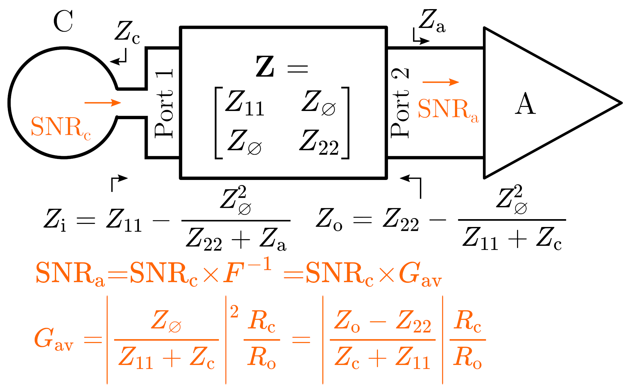
Figure 1. A lossy matching network is inserted between a coil C and a preamplifier A. The network has an impedance matrix \(\mathbf{Z}\). The network presents \(Z_\mathrm{o}\) to A at the design frequency. The network presents \(Z_\mathrm{i}\) to coil C for the minimum current at the design frequency. The matching network has available power gain \(G_{\mathrm{av}}\) and noise figure \(F=G_{\mathrm{av}}^{-1}\) at 290 K.4 The SNR at coil C is degraded by \(F\) after passing through the matching network before entering preamplifier A. Unless otherwise noted, \(R=\Re Z\), \(X=\Im Z\).
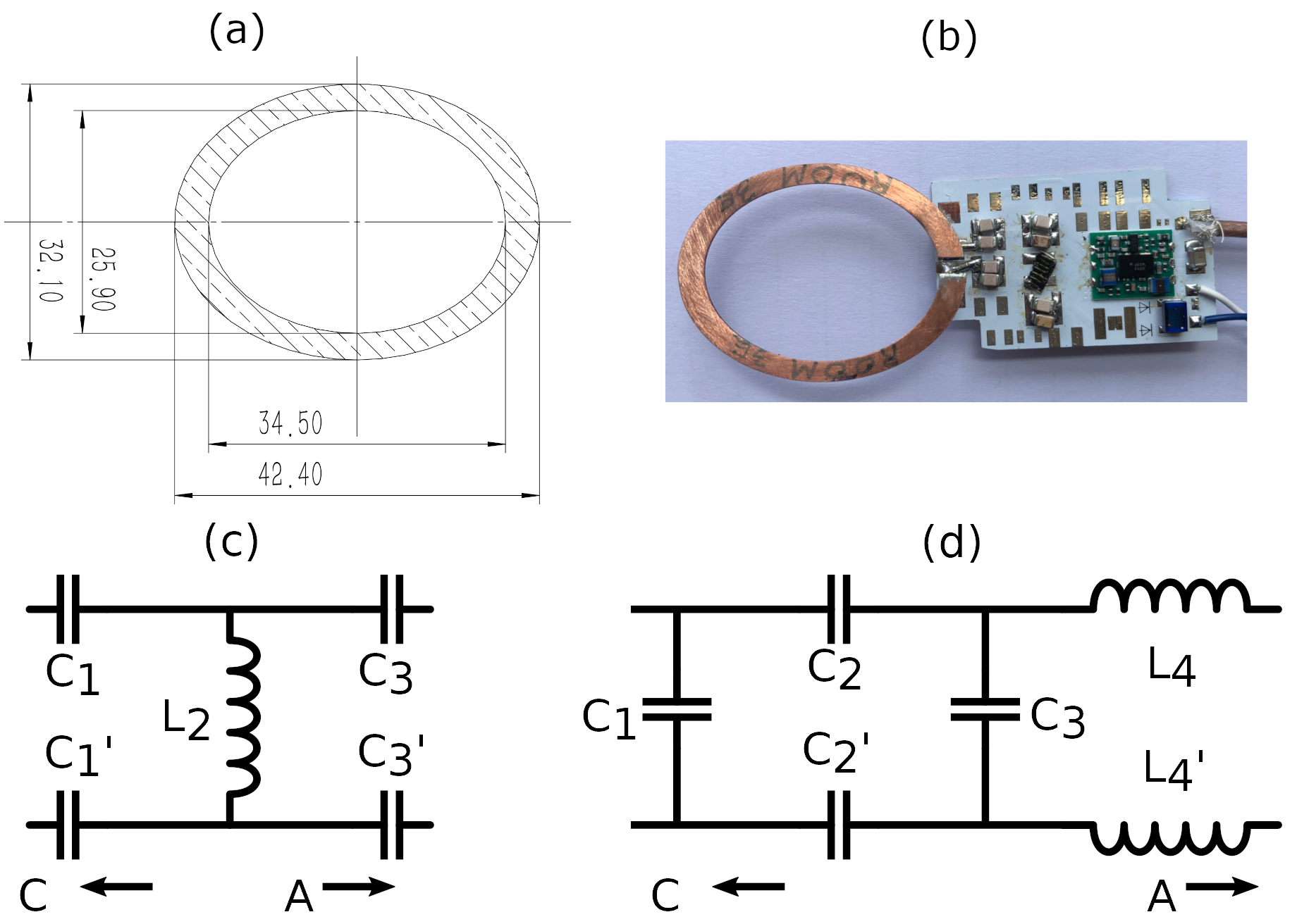
Figure 2. (a)
Dimensions of the coil in mm. (b) A fabricated PCB. Active decoupling circuitry
is not installed for simplicity of experiment. (c) The three-element matching
network. (d) The four-element matching network.
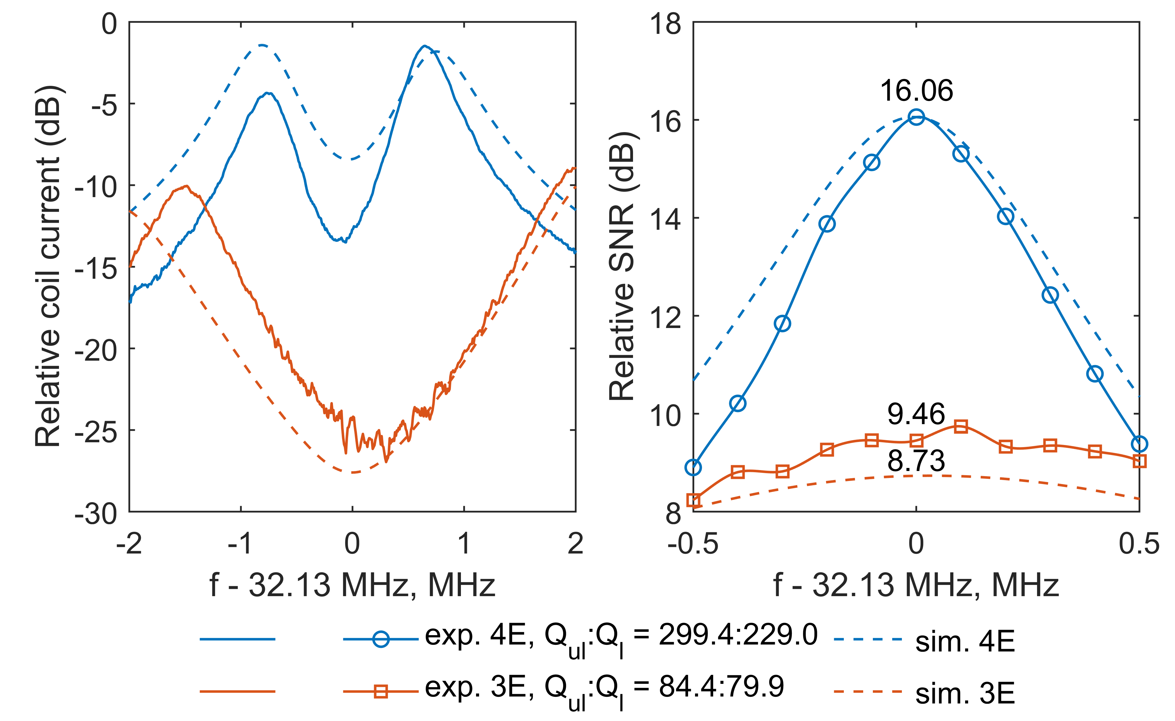
Figure 3. Measured and simulated coil current and SNR. The four-element ('exp. 4E') network gives ratio of unloaded Q to loaded Q as \(Q_{\mathrm{ul}}:Q_\mathrm{l} = 299.4:229.0\). The three-element ('exp. 3E') network gives \(Q_{\mathrm{ul}}:Q_\mathrm{l} = 84.4:79.9\). The SNR of the four-element network is higher than the SNR of the three-element network by 6.60 dB at 32.13 MHz. The simulated curves differ from measured curves mainly because coil Q and capacitor Q are high so that simulation, especially of coil current, is prone to errors.
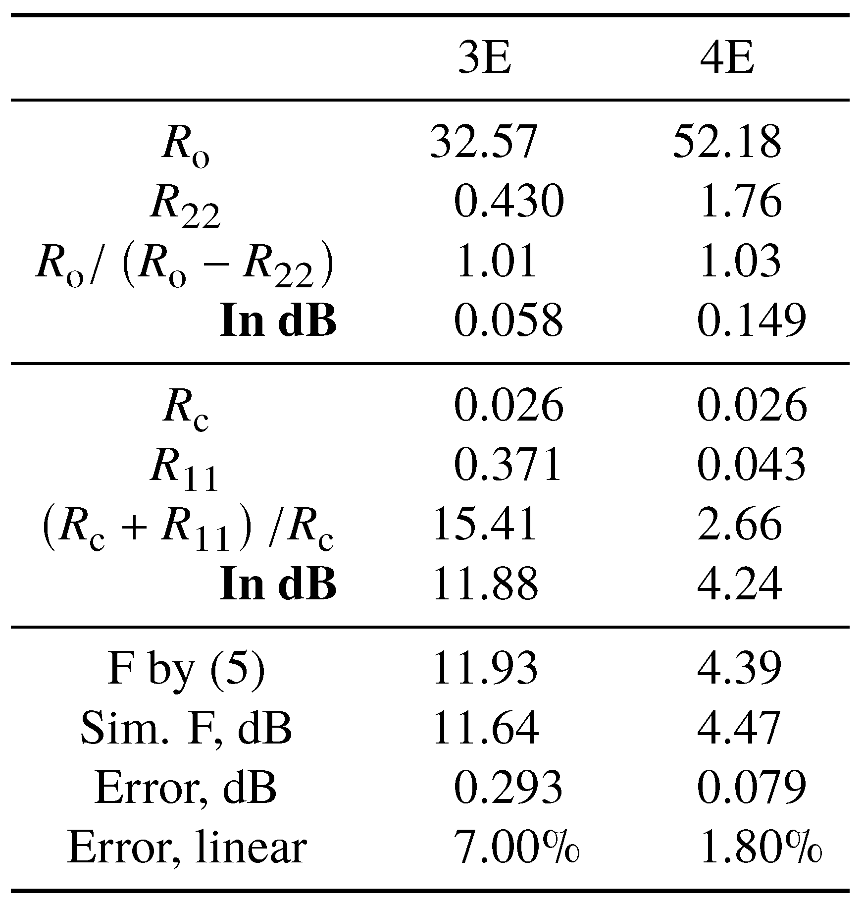
Figure 4. Decomposition of \(F\) for the three- ('3E') and four-element ('4E') matching networks using \(R_{11}\), \(R_{22}\), \(R_\mathrm{o}\), \(R_\mathrm{c}\) from Advanced Design System's layout simulation. There can be some rounding error in numbers. 'Sim. F' is the \(F\) given by Advanced Design System. 'Error' is the difference between 'F by (5)' and 'Sim. F'. It is seen that (5) estimates \(F\) accurately, and the major SNR-degrading term is \(\left( R_\mathrm{c} + R_{11} \right)/R_\mathrm{c}\).
DOI: https://doi.org/10.58530/2023/3905