Synopsis

Keywords: Machine Learning/Artificial Intelligence, Image Reconstruction

Magnetic resonance cholangiopancreatography suffers from long examination times and artifacts originating from residual motion. To shorten the acquisition protocol, we acquired data at 12-fold undersampling and investigated a 3D Variational Network (VN) architecture for reconstruction. We compared a self-supervised training scheme and a supervised network trained on synthetic data. We find that the self-supervised method is only able to provide competitive reconstructions if the network is initialized with pre-trained weights, and even then does not offer superior performance over the supervised approach. For the presented exemplary data, the supervised VN showed comparable image quality as a reference Compressed Sensing model.

Purpose

Magnetic resonance cholangiopancreatography (MRCP) is the clinical gold standard for imaging the biliary tract with a heavily T₂-weighted acquisition. To prevent breathing motion from corrupting the acquisition, respiratory gating is employed. However, this makes the procedure time-consuming and prone to corruption from gating errors.

At the same time, artificial neural networks have recently been established for the reconstruction of undersampled MR data from accelerated exams. In particular, unrolling a gradient descent iteration has shown promising performance [1–3]. However, the need for large training datasets in classical supervised training can pose a major challenge for many potential applications. To circumvent this, self-supervised approaches have recently been proposed [4].

In the following, we investigate the feasibility of data-driven reconstruction of an accelerated MRCP protocol by a 3D Variational Network, using both a self-supervised and a supervised approach, and compare it to model-based Compressed Sensing reconstruction.

Methods

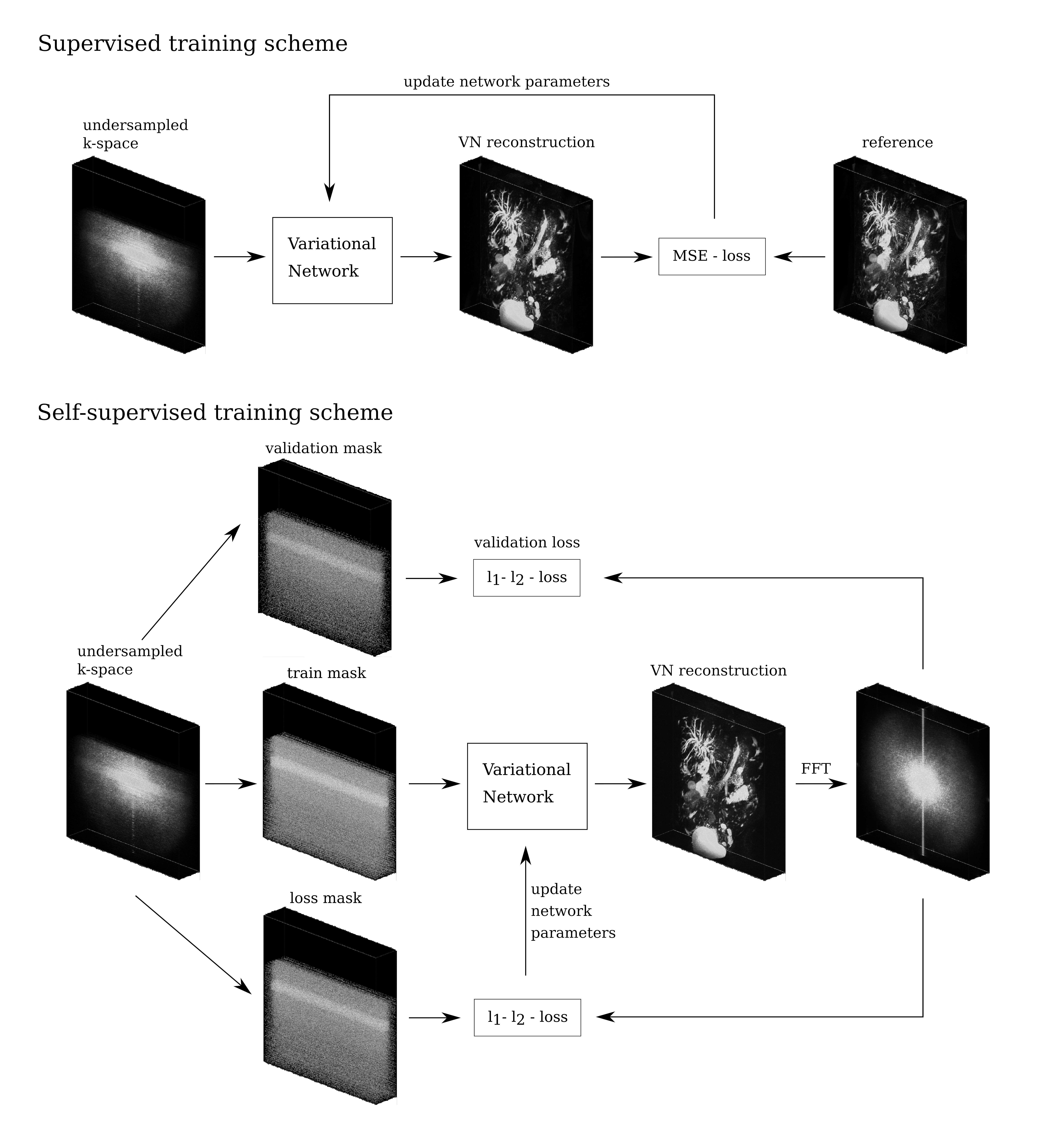
To test the subsequently presented approach, two prospectively undersampled MRCP datasets (R=12), as routinely acquired in our department at 3 T (Siemens Magnetom Prisma) with a CS-accelerated 3D fast spin echo sequence were exported. A Poisson-disk pattern and Partial Fourier sampling were used.

For reconstruction of these data, a Variational Network (VN) [1] with 3D architecture was employed. The unrolled gradient descent scheme featured 20 cascades, each comprising the enforcement of data consistency and application of a 3D U-Net. The VN was trained in a supervised and a self-supervised fashion:

For the supervised training, we used a dataset of 807 clinical 3D MRCP image series exported from our picture archiving and communication system. From these magnitude reconstructions, synthetic complex valued multi-coil k-space data was produced by using randomly generated coil sensitivity maps. Undersampling masks were then applied, resulting in a retrospectively undersampled, synthetic training dataset. With 81 volumes reserved for validation, these data were then used to train the VN in a classical supervised fashion for 16 epochs.

For the self-supervised training, we used an approach similar to [4]. For a given dataset, the sampled k-space positions are partitioned into three disjoint sets. The sampled data in the training set are used to generate a reconstruction. The predicted entries at k-space positions in the loss set are then compared to the measured data using a normalized $$$l_1$$$-$$$l_2$$$-loss function, to provide a loss for training the VN. The loss on the validation set is additionally computed to detect overfitting. An illustration of both training schemes can be seen in Fig.1.

The weights of the VN are initialized randomly before training. To combine the supervised and self-supervised methods, we additionally repeated the self-supervised training after initializing the VN with the weights from the supervised method. For additional comparison, we reconstructed the data with a Total Variation and $$$l_1$$$-wavelet-regularized Compressed Sensing (CS) model [5].

Results

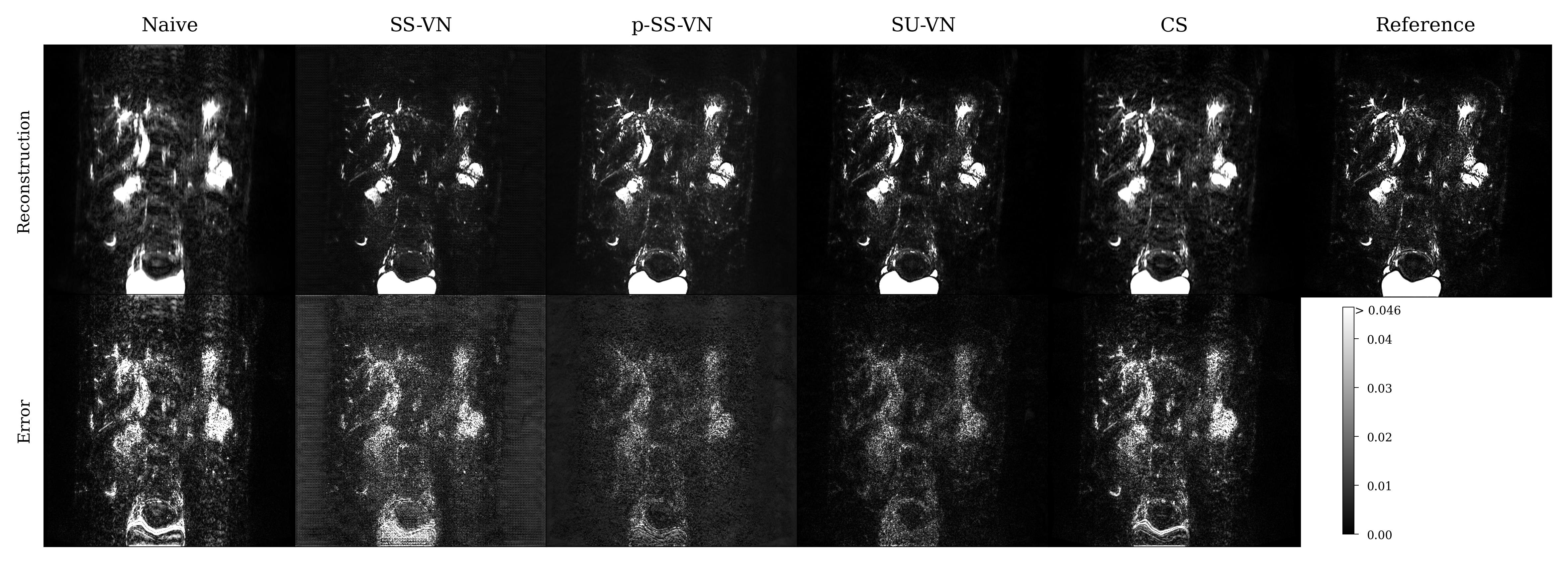
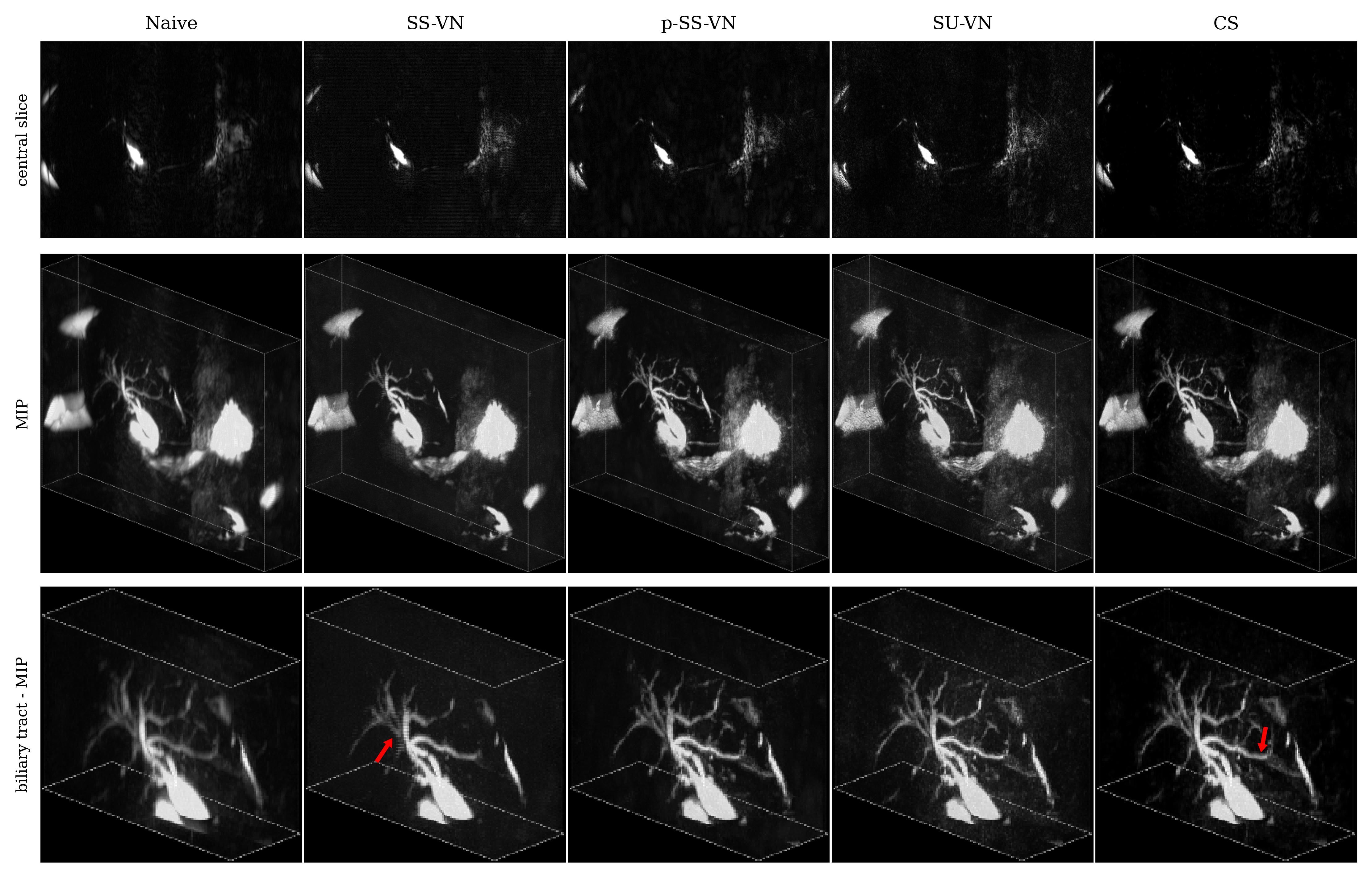
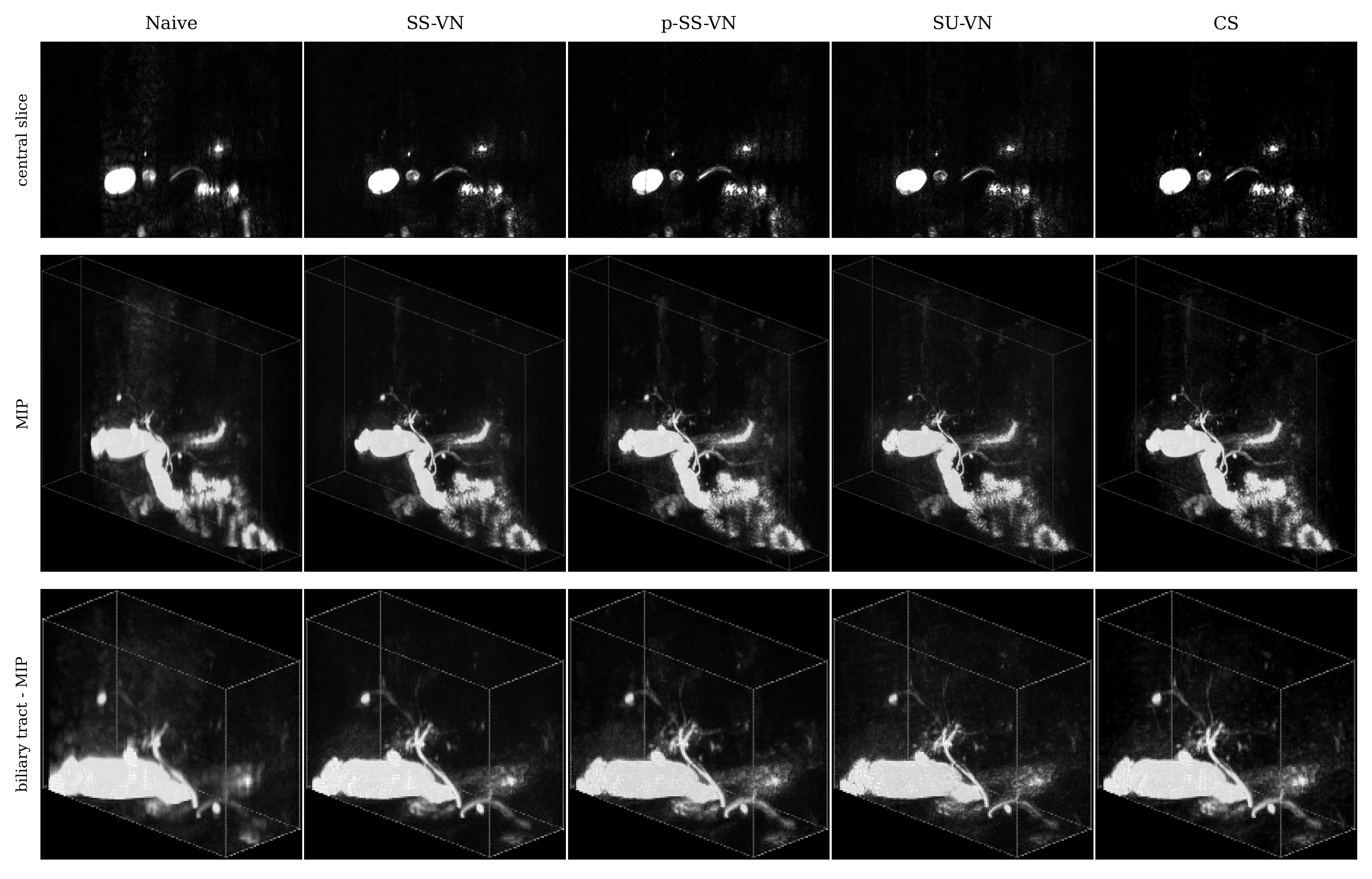
We first compared the described methods on a synthetic dataset, especially to be able to generate error maps (see Fig. 2). The self-supervised VN (SS-VN) reduces blurring effectively, but suffers from substantial artifacts which were introduced by the reconstruction. These are not present if the VN is initialized with pre-trained weights (p-SS-VN). The supervised VN (SU-VN) shows the lowest errors, overall sharpest appearance, and the least remaining artifacts in the reconstruction. The error of the CS reconstruction is higher, and blurring can be observed visually.

A comparison of the methods on prospectively undersampled data can be seen in Fig. 3 and 4. In SS-VN, artifacts are visible, and anatomical details are lost. This is much improved in p-SS-VN, where anatomy appears sharp, and substantially more details are visible. Noise is reduced considerably compared to SU-VN. The highest level of details can be seen in SU-VN and CS. SU-VN shows some remaining noise, while CS exhibits slight blurring.

Discussion & Conclusion

With random initialization, the self-supervised method performs poorly. This could be due to the amount of training data being too small or the acceleration factor being too high. If initialized with pre-trained weights, the self-supervised approach provides reconstructions with reduced noise, but also a slight loss of details w.r.t. SU-VN. However, the self-supervised method takes much longer, on the order of hours, while SU-VN and CS provide the reconstructions in just seconds. We conclude that for the application at hand, the noise reduction that the presented self-supervised method offers over the supervised method cannot be justified when considering the long reconstruction times and – more striking - the slight loss of details.

The supervised VN on the other hand performed well, with lower error and blurring compared to CS for the synthetic test dataset. For prospectively undersampled data, blurring was lower for VN too, however, slightly lower SNR compared to the CS reconstruction leaves the comparison at least partially inconclusive. A larger study with more test samples will possibly provide a clearer picture.

Authentic rawdata, i.e. complex-valued multi coil samples, could further benefit the generalization of the reconstruction model. However, collecting a training dataset of similar size as the one used here corresponds to significant effort, which is circumvented by the presented approaches.

Acknowledgements

Funding: German Ministry for Education and Research (BMBF), Research Grant 05M20WKA