3887
MRI Denoising with a Non-Blind Deep Complex-Valued Convolutional Neural Network
Quan Dou1, Zhixing Wang1, Xue Feng1, and Craig Meyer1
1Biomedical Engineering, University of Virginia, Charlottesville, VA, United States
1Biomedical Engineering, University of Virginia, Charlottesville, VA, United States
Synopsis
Keywords: Machine Learning/Artificial Intelligence, Machine Learning/Artificial Intelligence
Signal-to-noise ratio is crucial for MR image analysis. In this work, we proposed a non-blind complex-valued convolutional neural network for MRI denoising. Compared to existing denoising methods, the proposed method shows better performance on handling noise at different levels and on spatially variant noise.Introduction
MR images with high signal-to-noise ratio (SNR) provide more diagnostic information. The number of averages can be increased to obtain a higher SNR image, but this results in a longer scan time. On the other hand, images acquired on low-field scanners inherently have low SNR. In the past decade, various methods have been developed to reduce the noise in MR images1-3. However, most of them operate on the magnitude image and ignore that the collected MR signals are complex-valued. In this work, we trained a non-blind complex-valued convolutional neural network (CNN) with simulated data for MRI denoising. We then compared the results using the proposed method to results using state-of-the-art denoising methods.Methods
Ground truth images are required for supervised neural network training. Assuming a noise-free image $$$m(x)$$$, we generated the noise-corrupted image $$$m'(x)$$$ by applying random, complex, additive white Gaussian noise (AWGN) with zero mean and variance $$$\sigma_n^2$$$ to $$$m(x)$$$. The training and validation datasets used in this work were built from the fastMRI dataset4 (https://fastmri.med.nyu.edu/). We randomly selected 2000 T2-weighted imaging volumes for training the model and selecting model hyperparameters. During the noise simulation, each image was normalized to have its magnitude between 0 and 1 and its phase unchanged, and the noise standard deviation $$$\sigma_n$$$ was sampled from a uniform distribution between 0.04 to 0.08.A DnCNN5 was used as our backbone network structure. Instead of splitting the real and imaginary components into two separate channels, complex-valued operations were utilized throughout the network. The proposed non-blind $$$\mathbb{C}$$$DnCNN for MRI denoising is depicted in Figure 1. The input to the network was a 2D complex-valued MR image concatenated with a tunable complex-valued noise level map. The non-blind $$$\mathbb{C}$$$DnCNN consists of a series of complex-valued convolution blocks. Three types of operations were adopted in each block: complex-valued convolution ($$$\mathbb{C}$$$Conv)6, radial batch normalization (BN)7, and complex-valued rectified linear unit ($$$\mathbb{C}$$$ReLU)6. The network was implemented in PyTorch8 and trained with an L1 loss. The optimization was carried out by an Adam optimizer9 with an initial learning rate of 0.0001 and momentum parameters $$$\beta_1$$$ = 0.9 and $$$\beta_2$$$ = 0.999.
To evaluate the performance of the proposed denoising method, another 200 T2-weighted imaging volumes were randomly selected to avoid overlap between the training and testing subsets. Simulated AWGN with zero mean and standard deviation between 0 to 0.1 was added to the testing data. We compared our method with other denoising algorithms including non-local means (NLM) filter1, Block-matching and 3D filtering (BM3D)2, DnCNN with two-channel input, CDnCNN without noise level map (blind). NLM and BM3D were applied to the magnitude images, while the CNN-based methods were applied to the complex-valued images. For quantitative assessment, the normalized root-mean-square error (NRMSE), peak signal-to-noise ratio (PSNR), and structural similarity index (SSIM) of the magnitude images were calculated. We also explored the role of the noise level map in dealing with spatially variant noise in parallel imaging. In SENSE reconstruction10, the noise is amplified by the geometry factor (g-factor), which is dependent on the coil geometry. The g-factor map is calculated during the reconstruction and does not require additional scan time. We used the scaled g-factor map as the noise level map. Additionally, T1-weighted and FLAIR brain images and proton density (PD) weighted knee images from the fastMRI dataset were randomly selected to form a testing dataset out of the training distribution, which was used to test the generalizability of the model.
Results
Figure 2A shows the quantitative evaluation results at different noise levels. The proposed non-blind $$$\mathbb{C}$$$DnCNN outperforms other methods with lower NRMSE, and higher PSNR and SSIM. Figure 2B shows representative slices from the testing dataset. The output of non-blind $$$\mathbb{C}$$$DnCNN shows reduced noise and less visual blurring compared to other methods. The computational cost for each method is summarized in Table 1. Figure 3 shows the network performance on SENSE reconstructed image. With scaled g-factor map as the noise level map, non-blind $$$\mathbb{C}$$$DnCNN successfully removed the spatially variant noise, while other methods failed at the center regions with large g-factor. Figure 4 shows the network performance on testing data out of the training distribution. The network is able to denoise the images and shows good generalization capability.Discussion
This work demonstrates that a non-blind complex-valued CNN is capable of denoising MR images. The proposed method outperforms real-valued DnCNN and conventional denoising methods such as NLM and BM3D. With the additional information from the noise level map, the network provides the flexibility to handle noise at different levels, and spatially variant noise. The method can be used to improve the SNR of the images acquired with low-field scanners.Acknowledgements
The authors acknowledge support from Siemens Medical Solutions.References
[1] Manjón JV, Carbonell-Caballero J, Lull JJ, García-Martí G, Martí-Bonmatí L, Robles M. MRI denoising using non-local means. Med Image Anal. 2008 Aug;12(4):514-523.[2] Makinen Y, Azzari L, Foi A. Collaborative Filtering of Correlated Noise: Exact Transform-Domain Variance for Improved Shrinkage and Patch Matching. IEEE Trans Image Process. 2020 Aug 12;PP.
[3] Koonjoo N, Zhu B, Bagnall GC, Bhutto D, Rosen MS. Boosting the signal-to-noise of low-field MRI with deep learning image reconstruction. Sci Rep. 2021 Apr 15;11(1):8248.
[4] Zbontar J, Knoll F, Sriram A, et al. fastMRI: An Open Dataset and Benchmarks for Accelerated MRI. 2018. arXiv:1811.08839 [cs.CV].
[5] Zhang K, Zuo W, Chen Y, Meng D, Zhang L. Beyond a Gaussian Denoiser: Residual Learning of Deep CNN for Image Denoising. IEEE Trans Image Process. 2017 Jul;26(7):3142-3155.
[6] Trabelsi C, Bilaniuk O, Zhang Y, et al. Deep complex networks. 2018. arXiv:1705.09792 [cs.NE].
[7] El-Rewaidy H, Neisius U, Mancio J, Kucukseymen S, Rodriguez J, Paskavitz A, Menze B, Nezafat R. Deep complex convolutional network for fast reconstruction of 3D late gadolinium enhancement cardiac MRI. NMR Biomed. 2020 Jul;33(7):e4312.
[8] Paszke A, Gross S, Massa F, et al. Pytorch: An imperative style, high-performance deep learning library. 2019. arXiv:1912.01703 [cs.LG].
[9] Kingma D, Ba J. Adam: A method for stochastic optimization. 2014. arXiv:1412.6980 [cs.LG].
[10] Pruessmann KP, Weiger M, Scheidegger MB, Boesiger P. SENSE: sensitivity encoding for fast MRI. Magn Reson Med. 1999 Nov;42(5):952-62.
Figures
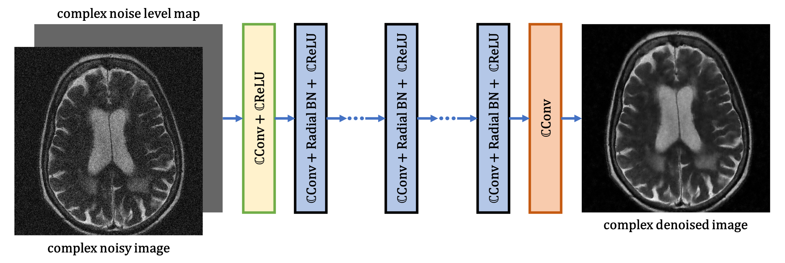
Figure 1 Architecture of the proposed non-blind $$$\mathbb{C}$$$DnCNN.
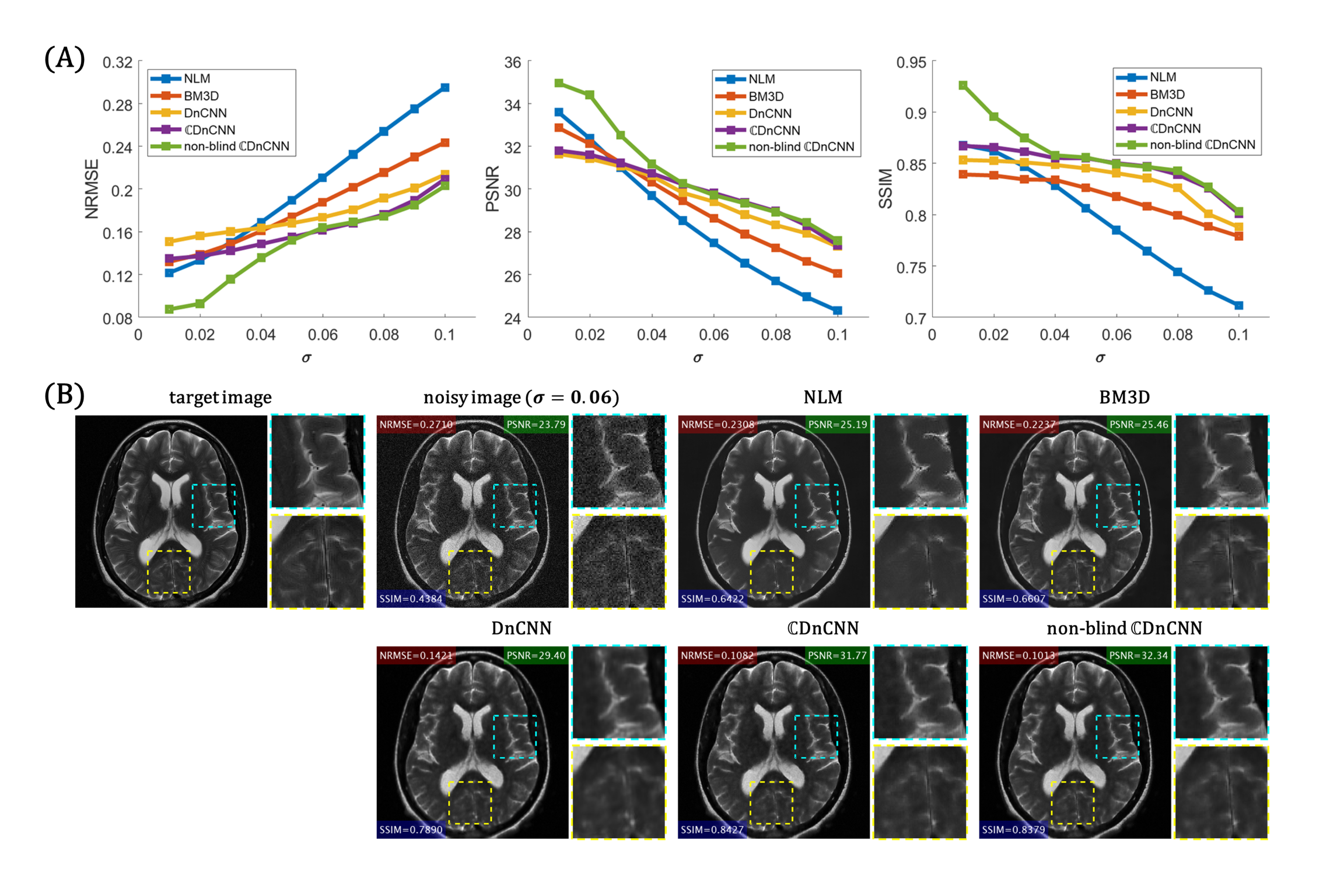
Figure 2 (A) Quantitative evaluation results at different noise levels. (B) Representative slices from the testing dataset.
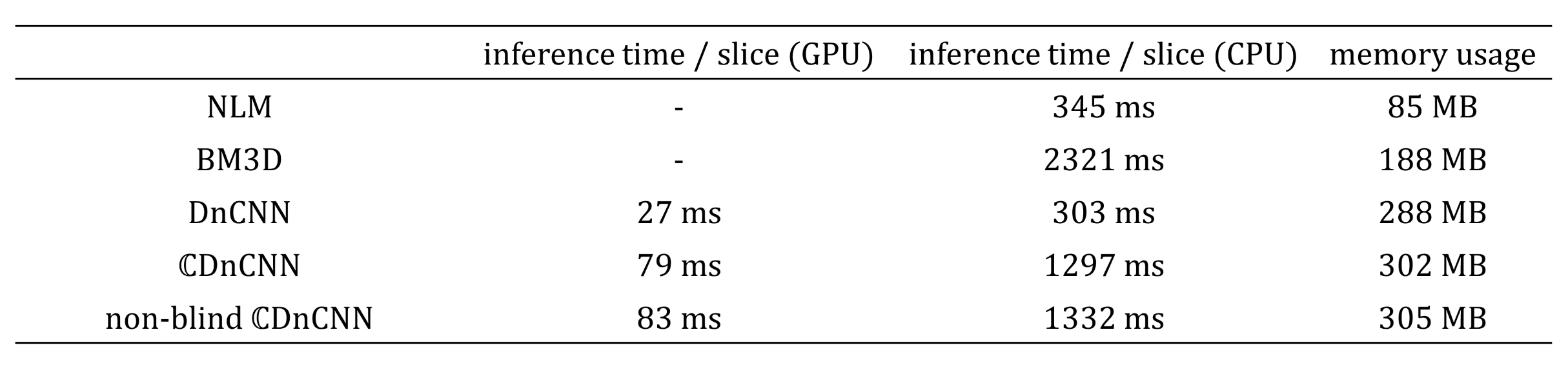
Table 1 Computational cost for different denoising methods.
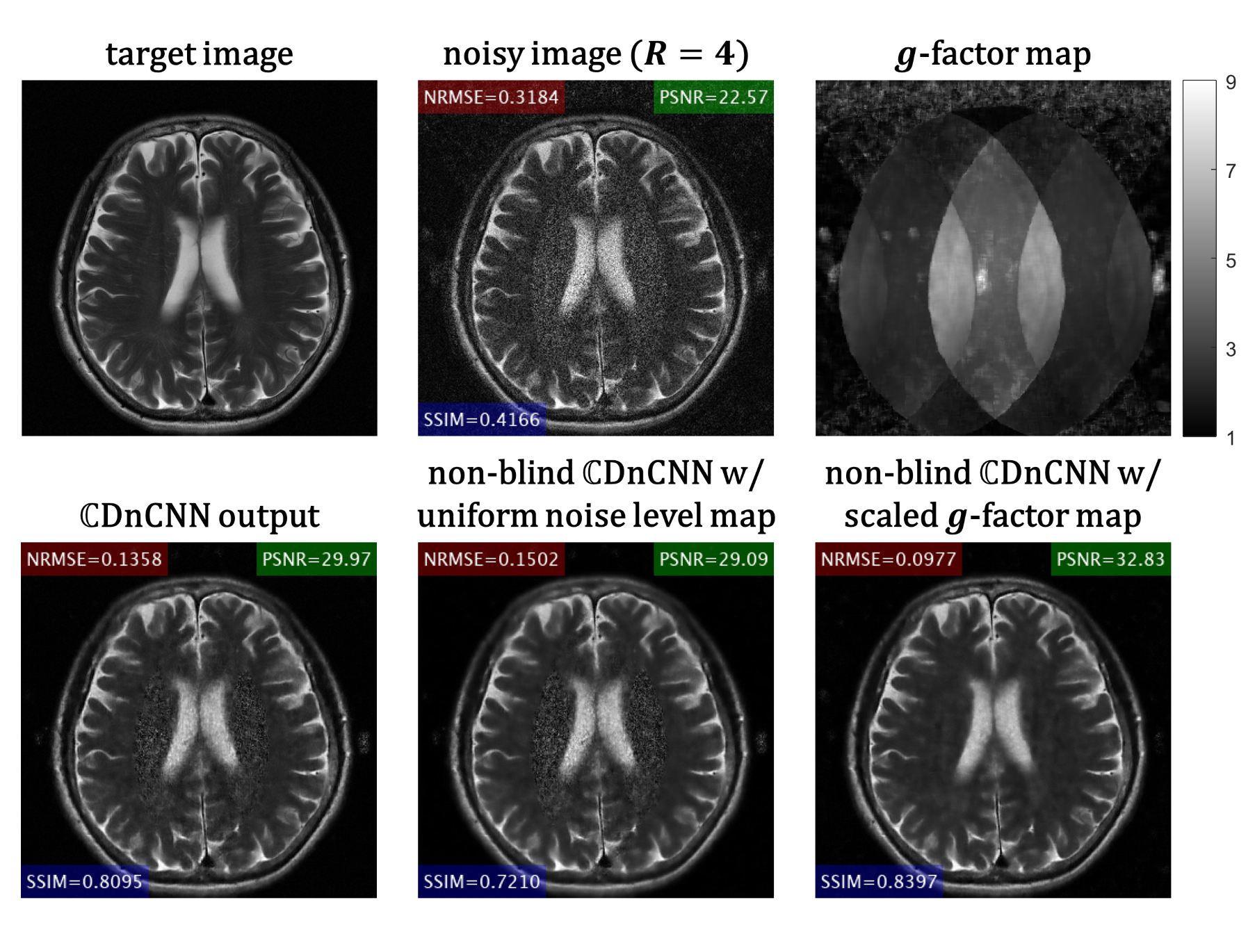
Figure 3 Network performance on SENSE reconstructed image with spatially variant noise.
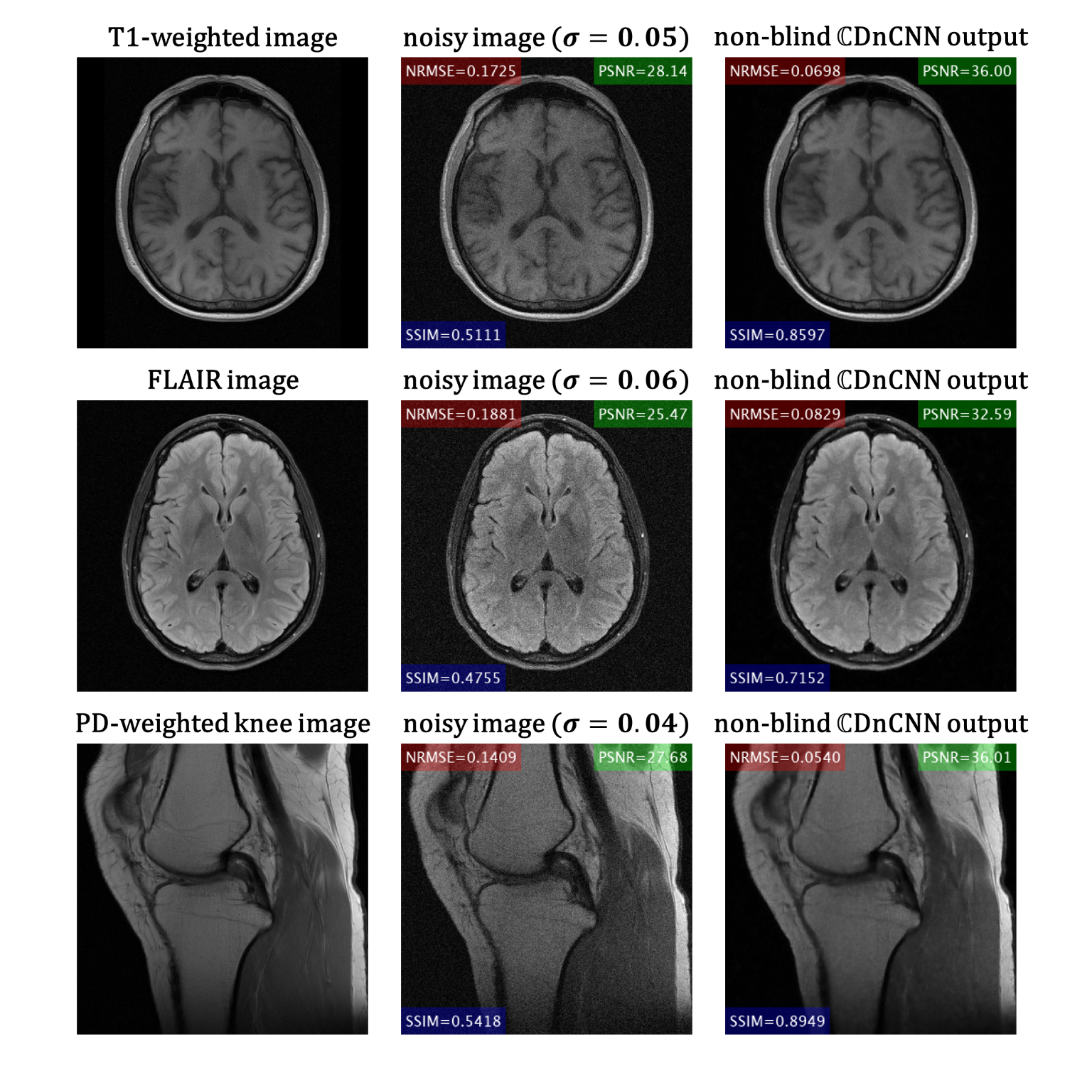
Figure 4 Representative slices from the testing dataset out of the training distribution.
DOI: https://doi.org/10.58530/2023/3887