3877
Super-Resolution Reconstruction of CEST images for human brain at 3T based on deep learning1Center for Biomedical Imaging Research, Department of Biomedical Engineering, Tsinghua University, Beijing 100084, China, Beijing, China, 2Xi’an Key Lab of Radiomics and Intelligent Perception, School of Information Sciences and Technology, Northwest University, Xi’an, Shaanxi 710069, China, Xi'an, China
Synopsis
Keywords: Machine Learning/Artificial Intelligence, CEST & MT, Super-resolution, Unrolled network, quantitation
CEST MRI suffers from the low resolution, leading to the disability to image small structures. We proposed a new optimization process adapting the CEST data form. Based on deep learning, our optimization flow is unfolded into an unrolled network for super resolution, termed as SC-Net. Besides, we introduced ROI-based normalization loss to guarantee quantitation accuracy. Results showed that SC-Net could reconstruct high-resolution image series and quantitative maps (PSNR = 44.27dB, CNR APTw = 41.79dB), when down sampling rate = 8. And the ROI-based normalization loss could calibrate errors. In conclusion, SC-Net has the potential to image small regions and acceleration.Introduction
Chemical exchange saturation transfer (CEST) imaging is a fast-growing molecular imaging method that allows indirect detection of several metabolites in vivo. CEST usually require acquisition of multiple saturation frequency offsets, each including a seconds-long saturation time and an immediate image readout at water frequency. To obtain acceptable contrast-to-noise ratio (CNR), the CEST images often suffer from low-resolution(LR), which hinders the application of CEST on imaging fine structure.For the advance in deep learning, image-based Super-resolution reconstruction (SRR) plays a key role in MRI to improve the image quality. [1-3] In this study, we proposed an unrolled deep learning network, termed as SC-Net, with ROI-based normalization loss to obtain high-quality high-resolution(HR) CEST series.
Method
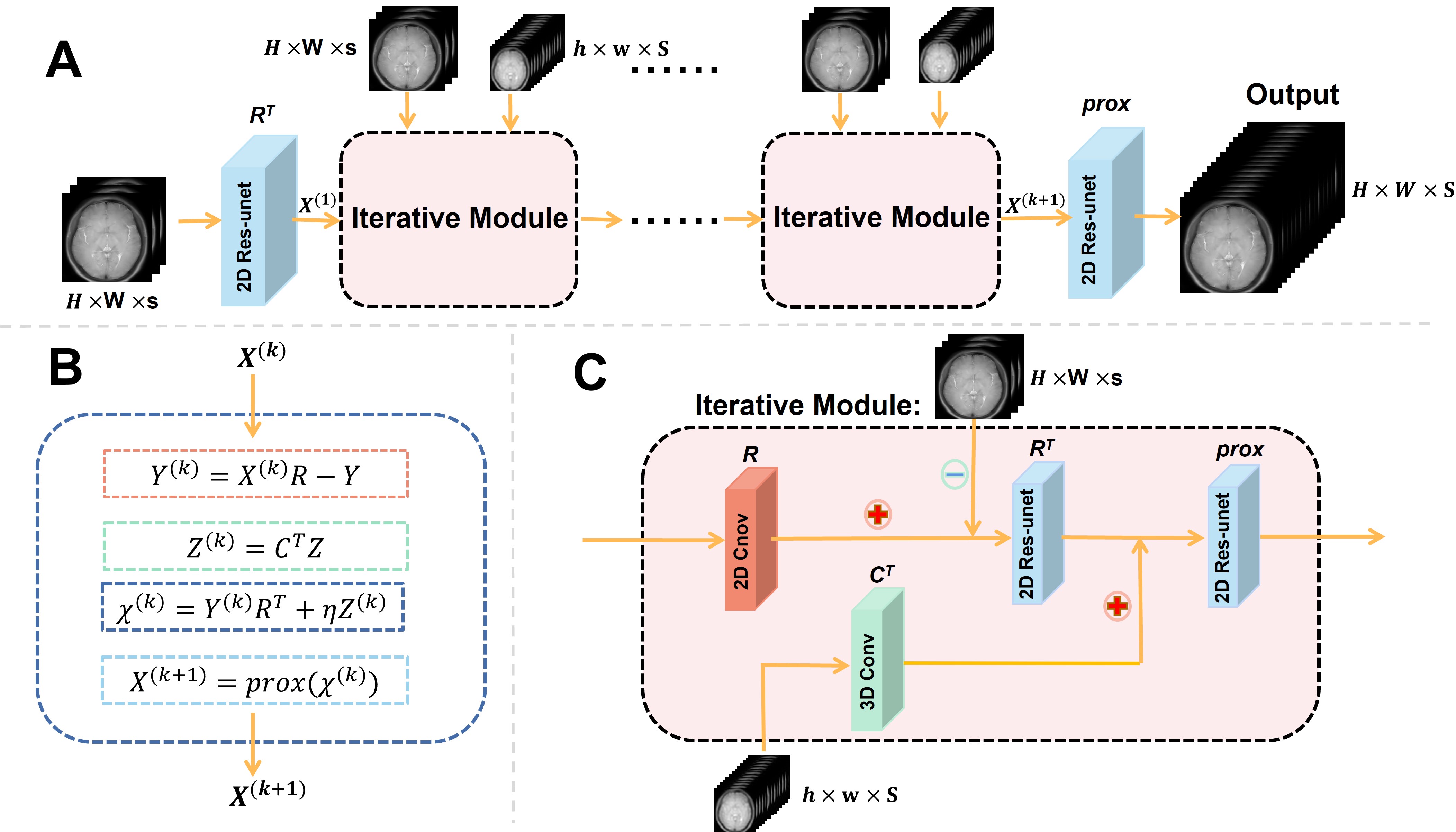
In this section, we first introduce the proposed optimization process and architecture of our SC-Net. Then, ROI-based normalization loss is also interpreted in detail.Network architecture: Diagram of the proposed optimization process and network is shown in Figure 1. We input several HR images and LR series with all Z-spectrum into the network to obtain fusion HR images series with all Z-spectrum. Based on corresponding optimization process adapting the CEST data form, we build iterative module, which ensure the reconstruction of CEST more accurate. R denotes the down-sampling Z-spectrum operator, in contrast, Rt denotes the up-sampling operator. Ct represents the spatial up-sampling operators. And we perform prox operator which represent the proximal gradient algorithm using 2D Res-unet. We also use the strategy of sharing parameters in several iterative modules, leading to our network similar to a recursive structure (RNN) and retaining information better.
ROI-based normalization loss: CEST quantitative analysis need to perform normalization, However, normalization will cause significant changes in the distribution of data. Therefore, we proposed the ROI-based normalization loss (RBN) to constrain the normalized image. $$RBN LOSS = {\textstyle \sum_{i=2}^{S}}\left | \frac{\chi _{i}\cdot M }{\chi _{1}}- \frac{X_{i}\cdot M }{X_{1}} \right |_{1}\cdot \frac{1}{S-1} $$
Where $$$\chi_i$$$ denotes the result of reconstruction, $$$X_i$$$ denotes the ground truth, $$$\chi_1$$$ and $$$X_1$$$ represent the S0 of output and truth for normalization, respectively. S represents the sampling point on Z-spectrum.M denotes the ROI-mask.
According to characteristics of our model, we use L1 to constrain the output of each stage in network, named model-based loss. Besides, we also introduce angle similarity loss which is widely used in measurement of spectrum similarity. Finally, our final loss is expressed as:$$loss=model\ based\ loss+\ \alpha\ast angle\ loss+\ \beta\ast RBN\ loss $$
Where $$$\alpha$$$ and $$$\beta$$$ are used as trade-off parameter.
Datasets: We totally used 2 datasets on human for training and evaluation. The first dataset is utilized to pre-train and warm-up the framework, and the formally training of framework, evaluation and following results are performed on Dataset 2. All experimental images were obtained from a Philips Ingenia CX 3T MR scanner (Philips Healthcare, Best, The Netherlands).
Dataset 1: 10 subjects were involved, collected for high-resolution CEST-MRI volumes. And the parameters are shown as follows: FOV = 192×192 mm2, resolution = 0.75×0.75 mm2, TR = 3500 ms, TE = 13 ms, B1=0.7 μT, number of slices = 20, slice thickness = 5 mm, SENSE = 4, 31 frequency offsets including S0 are collected.
Dataset 2: 8 high-resolution and the par 4-fold LR CEST-MRI volumes were collected from 7 health volunteers and 1 patient with vascular space dilation. The HR CEST scanning parameters: frequency offsets, TE, B1, resolution, FOV is the same as dataset 1. But others are modified for TR = 4000 ms, SENSE=1.6, number of slices = 12, slice thickness = 4mm. For LR CEST-MRI, only resolution = 3×3 mm2 differed from the HR images.
Results and Discussion
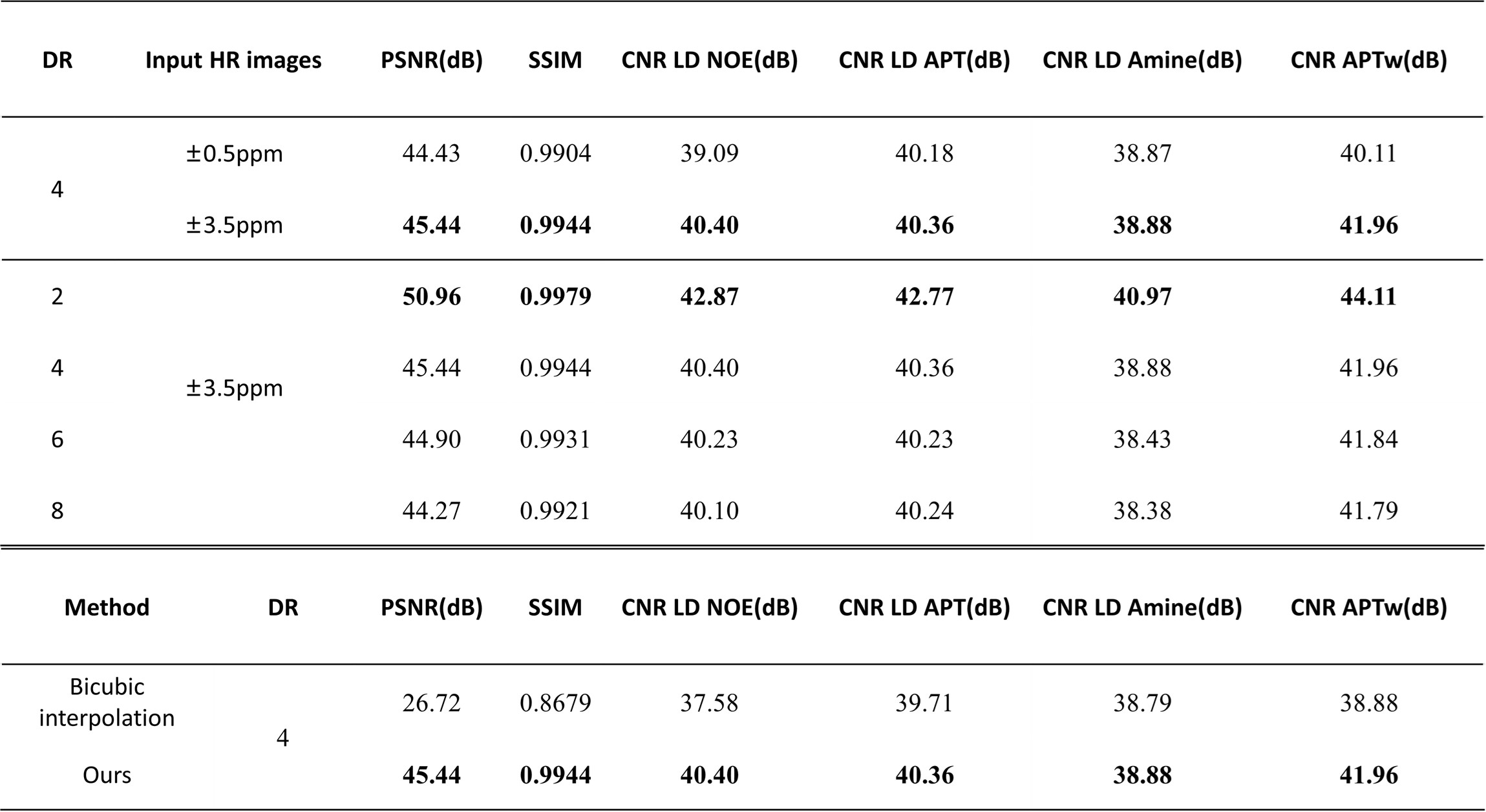
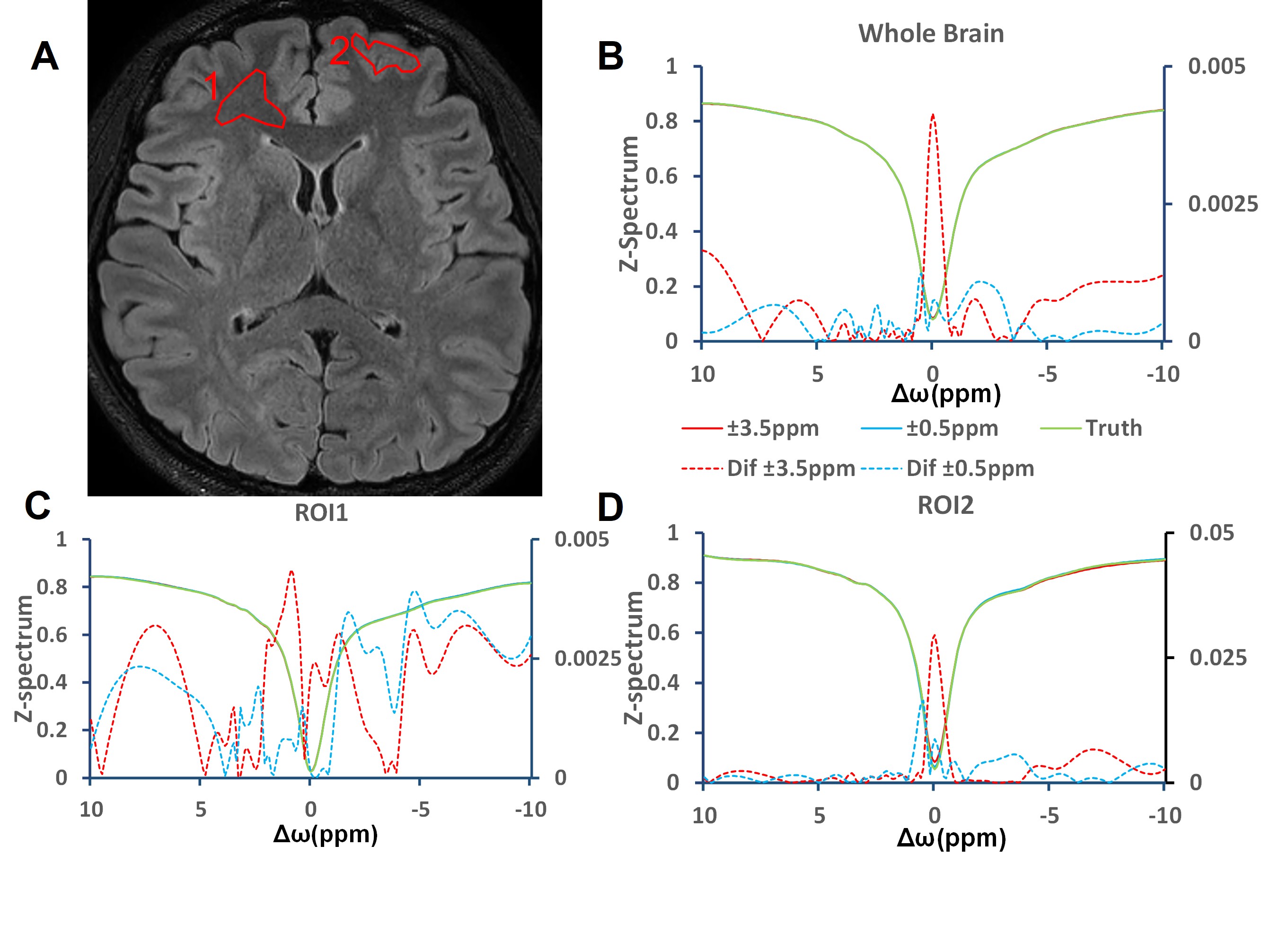
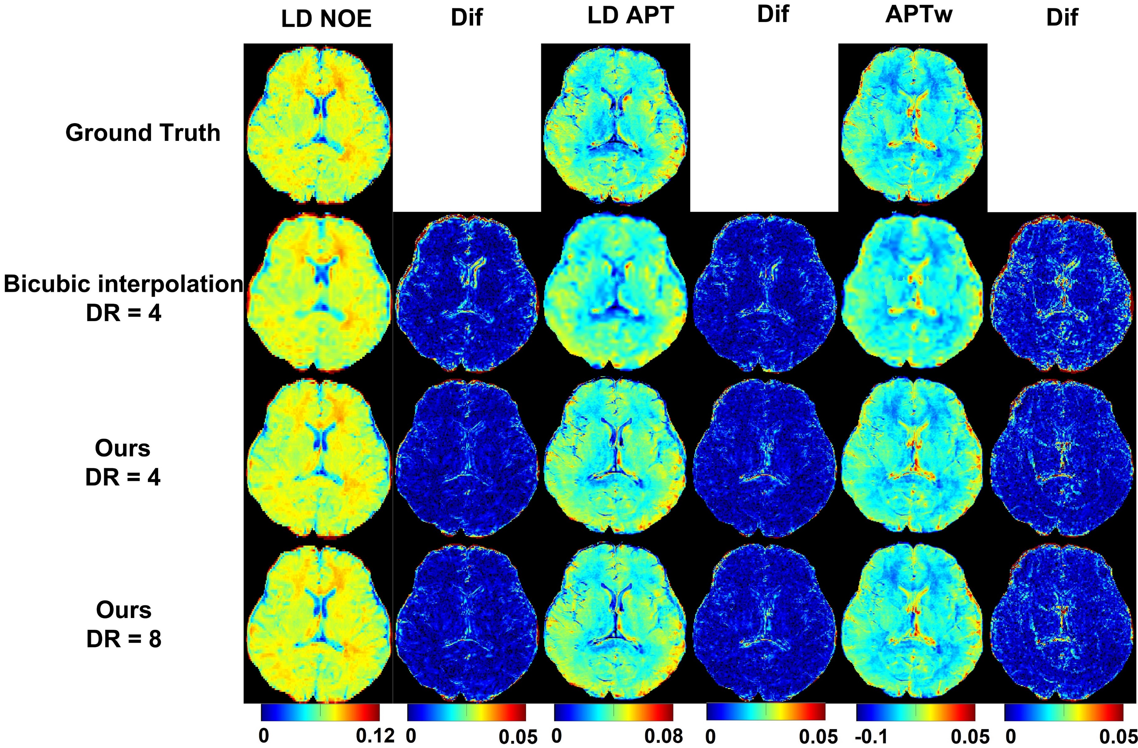
Retrospective study:First, in terms of iterative module number, we choose 3, which showed the best performance of network (PSNR = 45.44 dB). And when input HR are S0, ±3.5 ppm, the CNR is the highest in all quantitative maps and Z-spectrum, far better than when input HR images are ±0.5ppm(Figure 2, Table 1). Based on the former two experiments, we evaluated the network SR ability for different down-sampling rate (DR) (Figure 4). It is observed that with down-sampling rate increasing, error increases gradually but the spatial details are still retained even when DR = 8(PSNR = 44.27dB, SSIM = 0.9921, CNR of LD NOE = 40.10 dB, CNR of APTw = 41.79 dB), which indicates that network can learn mapping relation from LR to HR and complement the spatial information.
Prospective study:
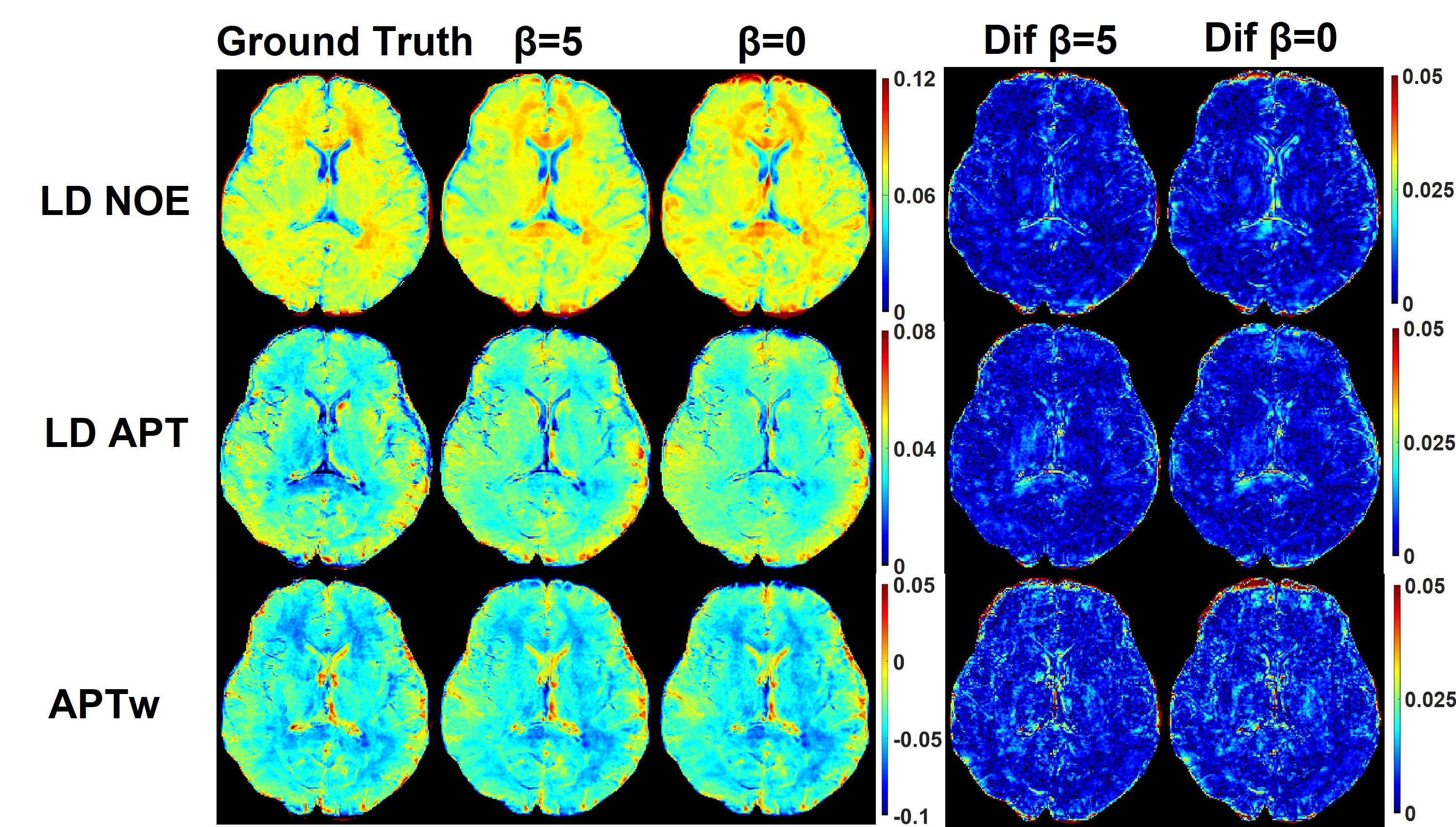
As shown in Figure 4, RBN loss displays capability to rectify the error especially near the edge of the whole brain and CSF. But prospective results are still inferior to retrospective study. This can be attributed to different data distribution and lack of prospective down sampling data for finely tuning network.
Conclution
The retrospective and prospective experiments show that proposed unfolded network SR-CEST with RBN loss may have the ability to reconstruct high-resolution CEST images series and have the potential on further reduction of scanning time based on the traditional acquisition acceleration methods such as SENSE, compress sensing.Acknowledgements
No acknowledgement found.References
[1] Cherukuri V, Guo T, Schiff S J, et al. Deep MR image super-resolution using structural priors[C] 2018 25th IEEE International Conference on Image Processing (ICIP). IEEE, 2018: 410-414.
[2] Lu Z, Li Z, Wang J, et al. Two-Stage Self-supervised Cycle-Consistency Network for Reconstruction of Thin-Slice MR Images[C] International Conference on Medical Image Computing and Computer-Assisted Intervention. Springer, Cham, 2021: 3-12.
[3] Tsiligianni E, Zerva M, Marivani I, et al. Interpretable Deep Learning for Multimodal Super-Resolution of Medical Images[C] International Conference on Medical Image Computing and Computer-Assisted Intervention. Springer, Cham, 2021: 421-429.
Figures