3875
Estimating Uncertainty of Deep Learning for Tomographic Image Reconstruction Through Local Lipschitz1Biomedical Engineering, Boston University, Boston, MA, United States, 2Athinoula A. Martinos Center for Biomedical Imaging, Charlestown, MA, United States, 3Google, Mountain View, CA, United States, 4Biostatistics, Harvard University, Cambridge, MA, United States, 5Harvard Medical School, Boston, MA, United States, 6Physics, Harvard University, Boston, MA, United States
Synopsis
Keywords: Machine Learning/Artificial Intelligence, Image Reconstruction
As deep learning approaches for image reconstruction become increasingly used in the radiological space, strategies to estimate reconstruction uncertainties become critically important to ensure images remain diagnostic. We estimate reconstruction uncertainty through calculation of the Local Lipschitz value, demonstrate a monotonic relationship between the Local Lipschitz and Mean Absolute Error, and show how a threshold can determine whether the deep learning technique was accurate or if an alternative technique should be employed. We also show how our technique can be used to identify out-of-distribution test images and outperforms baseline metrics, i.e. deep ensemble and Monte-Carlo dropout.Introduction
All imaging modalities from ultrasound to magnetic resonance imaging (MRI) employ tomographic image reconstruction techniques, i.e. the conversion of sensor domain data to the image domain. DL for tomographic image reconstruction has shown huge promise in solving inverse problems of this type, particularly in the medical field. Since the goal is to perform a diagnostic task, the reconstruction needs to occur with high confidence due to the health risk to patients. Thus, it is critical to estimate the uncertainty of deep learning (DL) for tomographic image reconstruction techniques in practice so that we know the reconstruction occurred appropriately. We propose calculating the Local Lipschitz value to estimate model uncertainty. We demonstrate the monotonic relationship between the Local Lipschitz and Mean Absolute Error (MAE) and use it to determine a threshold $$$\Upsilon$$$, through selective prediction, below which the DL technique performed appropriately. We also demonstrate through perturbation of an input, similar to the Local Lipschitz calculation by adding noise, that we can identify out-of-distribution (OOD) test images and outperform baseline methods of deep ensemble and Monto-Carlo dropout.Materials and Methods
Using the AUTOMAP neural network1, we trained and tested 2D T1-weighted brain MR images acquired at 3T collected from the MGH-USC Human Connectome Project (HCP) public dataset2 as the in-distribution (ID) dataset. We used the NYU fastMRI knee images dataset3 as the OOD dataset. All test sets consist of 5,000 images.To measure the uncertainty of DL for tomographic image reconstruction tasks, we propose estimating the local Lipschitz constant. A function $$$f$$$ is $$$L$$$-Lipschitz continuous if for any input $$$x,y \in \mathbb{R}^{n}$$$, there exists a nonnegative constant $$$L \ge 0$$$.
$$\| f(x) - f(y) \| \le L \| x - y \|$$
To calculate the Local Lipschitz, we need to determine the upper bound caused by average case perturbations. Let us denote $$$\Phi$$$ for AUTOMAP, $$$L_{\Phi}$$$ for the Lipschitz constant, $$$x$$$ for input image, and $$$e$$$ for error. We can write the Local Lipschitz calculation from the above equation as follows.
$$\| \Phi(x+e) - \Phi(x) \| \le L_{\Phi} \| x+e-x \|$$
$$\| \Phi(x+e) - \Phi(x) \| \le L_{\Phi} * \| e \|$$
Given the small magnitude of $$$\|e\|$$$, we can reorganize the above equation and place an upper bound by empirically calculating $$$L_{\Phi}$$$, where image $$$x' = x + e$$$.
$$L_{\Phi} \ge \frac{\| \Phi(x') - \Phi(x) \|}{ \| x' - x \|}$$
Now we can calculate the $$$ L_{\Phi} $$$ for any image after we perturb it by Gaussian noise $$$e$$$ and compare the variations in the output space over the input space. Through comparing the difference in output to difference in input, the $$$ L_{\Phi} $$$ value corresponds to how the network weights affect the output image reconstructed. In Fig 1a, we demonstrate the strong monotonic relationship between the Local Lipschitz and MAE and the table in Fig 1b shows the Spearman correlation values at each noise level. We observe as MAE increases, the $$$ L_{\Phi} $$$ increases. We also compare our method to detect OOD images to baselines methods of deep ensemble and Monto-Carlo dropout. For deep ensemble, we trained four AUTOMAP models and for Monto-Carlo dropout, we trained an AUTOMAP model with a dropout layer to output 50 images.
Results and Discussion
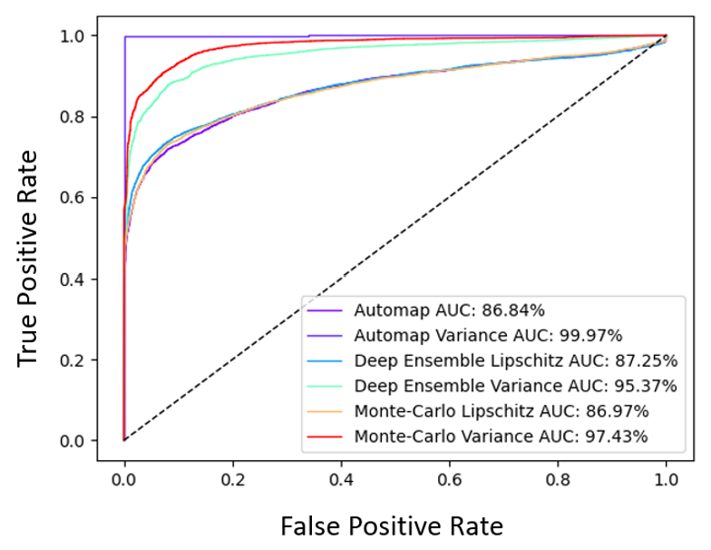
Fig 2a represents an image reconstruction pipeline where a threshold $$$\Upsilon$$$ can determine if the DL model or an alternative technique be used. If the Local Lipschitz is below $$$\Upsilon$$$, the DL performed with an appropriate accuracy. Otherwise, an alternative technique should be employed due to too large of an uncertainty. Fig 2b and 2c show how selective prediction is performed to determine $$$\Upsilon$$$ at different noise levels. The $$$L_{\Phi}$$$ was sorted in descending order with its corresponding MAE. The mean MAE decreases as more images with the highest $$$L_{\Phi}$$$ are referred. A radiologist can determine acceptable accuracy and a threshold based on the percentage referred. We also demonstrate how our method can be used to determine OOD images. In Fig 3, we display the receiver operating characteristic curves (ROC) and area under the curves (AUC) values of five different methods to detect OOD images from the ID validation dataset. Using the $$$L_{\Phi}$$$ values as signal, a single AUTOMAP model has AUC of 86.84% and performs comparably to the baseline methods with 87.25% for deep ensemble and 86.97% for Monto-Carlo dropout. The baseline methods output multiple images; thus, we can calculate variance and use as signal. For the single AUTOMAP model, we can generate four outputs by perturbing through adding noises of the same distribution to the input and calculate variance of the outputs. Using variance as signal, the AUTOMAP model outperforms all other methods with AUC of 99.97%. Thus, our perturbation method of using noise similar to the Local Lipschitz signal, can determine OOD images in a clinical setting better than baseline methods using only a single model.Conclusion
DL for tomographic image reconstruction has shown huge promise in solving inverse problems, particularly in the medical field. We provide a simple and scalable technique for estimating uncertainty through calculating the Local Lipschitz value, demonstrate its relationship to MAE and determine a threshold for using the DL model or not, and use it to detect OOD test images.Acknowledgements
We acknowledge support for this work from the National Science Foundation Graduate Research Fellowship under Grant No. DGE-1840990 and the NSF NRT: National Science Foundation Research Traineeship Program (NRT): Understanding the Brain (UtB): Neurophotonics DGE-1633516NSF.References
1. Zhu, Bo, et al. "Image reconstruction by domain-transform manifold learning." Nature 555.7697 (2018): 487-492.
2. Fan Q, Witzel T, Nummenmaa A, Dijk KRAV, Horn JDV, Drews MK, et al. MGH–USC Human Connectome Project datasets with ultra-high b-value diffusion MRI. Neuroimage 2016; 124: 1108–1114.
3. Zbontar J, Knoll F, Sriram A, Murrell T, Huang Z, Muckley MJ, et al. fastMRI: An Open Dataset and Benchmarks for Accelerated MRI. Arxiv 2018.
Figures
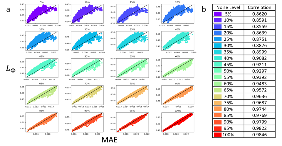

Fig 2: Reconstruction benchmark: A) represents the image reconstruction pipeline where a threshold $$$\Upsilon$$$ can determine if the DL model or an alternative technique be used. B and c) show how selective prediction is performed to determine $$$\Upsilon$$$ at different noise levels. The $$$L_{\Phi}$$$ was sorted in descending order with its corresponding MAE. The mean MAE decreases as more images with the highest $$$L_{\Phi}$$$ are referred. A radiologist can determine acceptable accuracy and a threshold based on the percentage referred.