3803
A NEW METHOD TO ANALYSE RENAL PERFUSION: A PROOF OF CONCEPT1Radiology, Ghent University Hospital, Ghent, Belgium, 2Diagnostic Sciences, Faculty of Medicine and Health Sciences, Ghent University, Ghent, Belgium, 3Ghent Institute of Functional and Metabolic Imaging, Ghent University, Ghent, Belgium, 4Nephrology, Ghent University Hospital, Ghent, Belgium, 5Internal Medicine and Pediatrics, Faculty of Medicine and Health Sciences, Ghent University, Ghent, Belgium, 66IBiTech– Medisip, Ghent University, Ghent, Belgium
Synopsis
Keywords: Kidney, Arterial spin labelling
To date, renal ASL MRI images are analysed with methods that may underestimate renal perfusion or that may be observer-dependent. In this study, we implemented two analysis methods that take into account the complex morphology of the kidney. One analyses the kidney progressively, from the cortex to the medulla, and the second one, a new algorithm analyses the kidney in radial sections. Our results show that perfusion values change across the kidney and that healthy subjects have higher perfusion values. This study shows the importance of using more robust analysis on kidney ASL MRI images.
Introduction
Consensus literature1,2 on renal ASL suggests the classical region of interest (ROI) analysis3. This method is observer-dependent4 and prone to variability. In healthy kidneys, is usually easy to differentiate kidney cortical and medullar region. Unfortunately, in non-healthy kidneys, this is more complex due to the anatomical degradation4. Piskunowicz et al. used the Concentric-Objects (CO) in blood oxygenation level-dependent (BOLD) images. In this paper, we tested the CO method in renal ASL images and, we implemented a new algorithm called Equiangular Object (EO) method, which allows for analysis along the renal cortex instead of perpendicular to the cortex. To date, renal ASL has been only analysed by classical ROI method5 and the histogram1,6 method. Therefore the goal is to test if these algorithms are comparable with these methods and if additional information might be retrieved.Methods
Thirteen subjects were scanned (7 healthy subjects, 6 patients) in a supine position on a Siemens PrismaFit 3T. The patient group conditions are resumed in Table 1. ASL images were obtained using a work-in-progress 3D Turbo Gradient Spin-Echo, pseudo-Continuous Arterial Spin Labeling (p-CASL) sequence (Siemens WIP 1023H), with voxel size: 3.8×3.8×5.0mm, TR/TE 5000/27.14ms, T1 Blood= 1650.0ms, Start TI=3000ms, PCASL duration 1500ms, PCASL flip-angle 28.0 deg. Perfusion was calculated inline using the classical compartment model. Both kidneys were segmented using FSLeyes. For each mask, the center of mass C(x,y) was calculated. Twelve-layer CO (TLCO) method classified each point P(x,y) inside the mask according to its distance (in 12 equal sections) to C. TLCO was implemented in Python and used to calculate mean perfusion values at different distances to the center. Consequently, a label image with 12 concentric layers was obtained.The EO method takes as input the C and all the points P inside the mask:1. Define a reference vector
a. Right kidney $$$\widehat{R_v}=(0,1)$$$
b. Left kidney $$$\widehat{L_v}=(0,-1)$$$
2. Define the vector between point P and center of mass: $$$\vec{v}=P-C$$$
3. Compute magnitude of vector ||v||.
4. Normalize vector $$$\widehat{v}= \frac{\vec{v}}{||v||}$$$
5. Compute the angle between points $$$\theta = atan2(\frac{v_xR_y-v_yR_x}{v_xR_x+v_yR_y})$$$
6. All points are sorted by the angle. If the points have the same angle, then shorter distance comes first.
7. The sorted points are divided in N groups, where N is the number of regions to classify the ROI
Ten regions are defined for the EO method. A label image with 10 equiangular object is obtained. TEO was used to calculate mean perfusion values across different sections of the kidney.
Results
One image for CO and EO method were computed. Mean RBF value of each layer/section was plotted to analyse the variation of RBF across the kidney. Healthy volunteers (HV)(N=7) were pooled to estimate a healthy profile for each kidney and compare it against patients. Figure.1 shows a healthy kidney in the process of generating the corresponding label images for the TLCO and TEO methods. Figure.2 shows the result of both methods in HV and in patients with chronic kidney disease (CKD)(N=2). [A1] In TLCO method, layer 0 is the outermost section of the kidney. In TEO method, 0 represents the lower pole of the kidney. TEO method shows in HV that perfusion is not constant along the cortex but is lower in both poles than in central sections of the kidney. Fig 3 shows the result of both methods in HV and transplant patients(N=2). The central section (segments 2-5) of right kidney is underperfused compared to the HV. Fig.4 shows the result of both methods in HV and the aorta aneurysm patient(N=1). The entire cortex is underperfused and the perfusion peak in the central section is not present. [A1]In table 1 I notice 2 patients with CKD and one with CNI (is CKD in dutch)Discussion
In literature, not all studies examine different regions of the kidney. RBF values in the cortex range between 2551-2905 mL/100g/min for HV and 716-831 mL/100g/min for patients. One study5 reported values for outer and inner medulla in HV of 91 ± 14 and 42 ± 16 mL/100g/min, respectively. For HV, the obtained values with TLCO method show higher RBF in outer layers and a decrease in the kidney inner region. This seems to be comparable with the results in literature. Looking the RBF values for the whole kidney in the literature, a value of 185.28-2287mL/100g/min is reported in HV, whereas a value of 94.68mL/100g/min is found for patients. The obtained values with the TEO method shows that RBF values in healthy subjects change from lower pole to upper pole of the kidney and that higher perfusion values are seen in the central section.Conclusion
Human kidney has a challenging geometry that requires robust algorithms to perform more complex analyses. Using only the mean of a region may underestimate different regional conditions of the kidney. The TEO and TLCO method results show that RBF values across the kidney change in different directions. By combining the TEO and TLCO method, or changing the number of layers and sections for both methods, an optimal configuration may be found depending on the application. Future applications include the use of the EO method to pinpoint underperfused areas in the kidney for more accurate steering of kidney biopsies.Acknowledgements
The authors thank Dr. Bernd Kühn (Siemens Healthcare AG, Erlangen, DE) for providing the ASL WIP sequence.References
1. Cox EF, Buchanan CE, Bradley CR, Prestwich B, Mahmoud H, Taal M, et al. Multiparametric Renal Magnetic Resonance Imaging: Validation, Interventions, and Alterations in Chronic Kidney Disease. Frontiers in physiology 2017;8:696.
2. Selby NM, Blankestijn PJ, Boor P, Combe C, Eckardt KU, Eikefjord E, et al. Magnetic resonance imaging biomarkers for chronic kidney disease: a position paper from the European Cooperation in Science and Technology Action PARENCHIMA. Nephrology, dialysis, transplantation : official publication of the European Dialysis and Transplant Association – European Renal Association 2018 Sep;33:ii4–ii14.
3. Nery F, Buchanan CE, Harteveld AA, Odudu A, Bane O, Cox EF, Derlin K, Gach HM, Golay X, Gutberlet M, Laustsen C, Ljimani A, Madhuranthakam AJ, Pedrosa I, Prasad PV, Robson PM, Sharma K, Sourbron S, Taso M, Thomas DL, Wang DJJ, Zhang JL, Alsop DC, Fain SB, Francis ST, Fernández-Seara MA. Consensus-based technical recommendations for clinical translation of renal ASL MRI. MAGMA. 2020 Feb;33(1):141-161. doi: 10.1007/s10334-019-00800-z. Epub 2019 Dec 12. PMID: 31833014; PMCID: PMC7021752.
4. Piskunowicz M, Hofmann L, Zuercher E, Bassi I, Milani B, Stuber M, et al. A new technique with high reproducibility to estimate renal oxygenation using BOLD-MRI in chronic kidney disease. Magnetic resonance imaging 2015 Apr;33:253–61
5. Eckerbom P, Hansell P, Cox E, Buchanan C, Weis J, Palm F, Francis S, Liss P. Multiparametric assessment of renal physiology in healthy volunteers using noninvasive magnetic resonance imaging. Am J Physiol Renal Physiol. 2019 Apr 1;316(4):F693-F702. doi: 10.1152/ajprenal.00486.2018. Epub 2019 Jan 16. PMID: 30648907.
6. Buchanan CE, Mahmoud H, Cox EF, McCulloch T, Prestwich BL, Taal MW, Selby NM, Francis ST. Quantitative assessment of renal structural and functional changes in chronic kidney disease using multi-parametric magnetic resonance imaging. Nephrol Dial Transplant. 2020 Jun 1;35(6):955-964. doi: 10.1093/ndt/gfz129. PMID: 31257440; PMCID: PMC7282828.
7. Gillis, K.A., McComb, C., Foster, J.E. et al. Inter-study reproducibility of arterial spin labelling magnetic resonance imaging for measurement of renal perfusion in healthy volunteers at 3 Tesla. BMC Nephrol 15, 23 (2014).
8. Cai YZ, Li ZC, Zuo PL, Pfeuffer J, Li YM, Liu F, Liu RB. Diagnostic value of renal perfusion in patients with chronic kidney disease using 3D arterial spin labeling. J Magn Reson Imaging. 2017 Aug;46(2):589-594
Figures
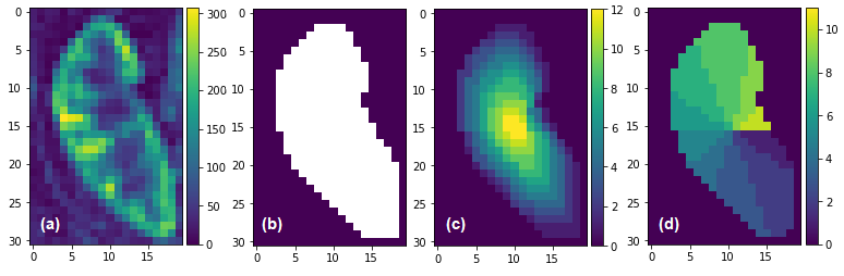
Fig. 1 (a) The RBF map from human kidney, (b) The mask image of the same kidney, (c) TLCO method applied to the mask image, (d) TEO method applied to the mask image
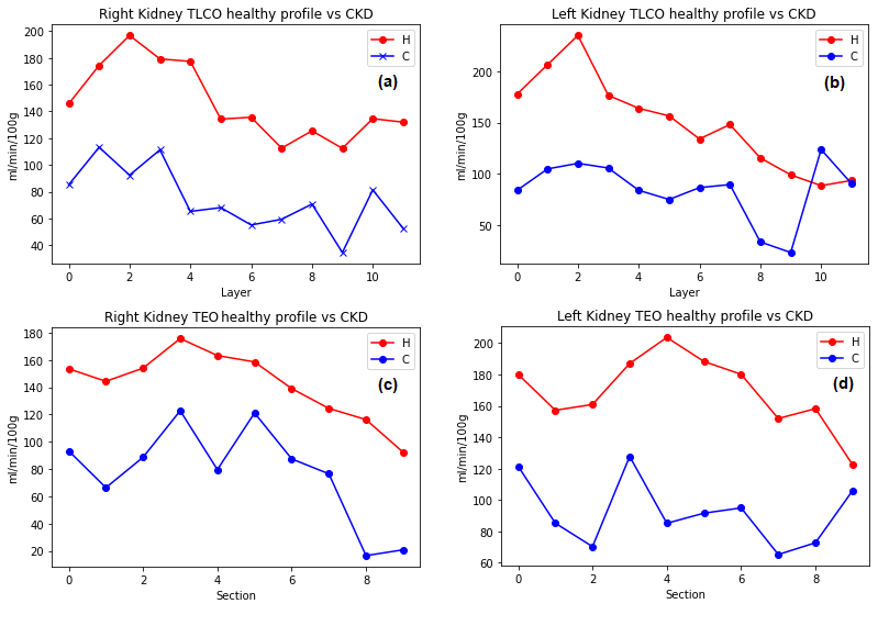
Fig. 2 Healthy volunteers profile vs CKD patients in (a) The TLCO right kidney, (b) The TLCO left kidney, (c) The TEO method in right kidney RBF, (d) The TEO method in left kidney RBF .
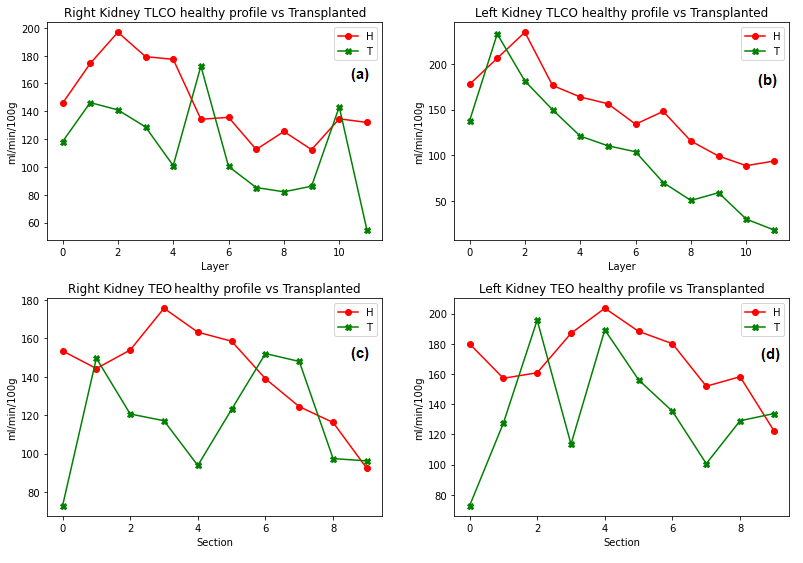
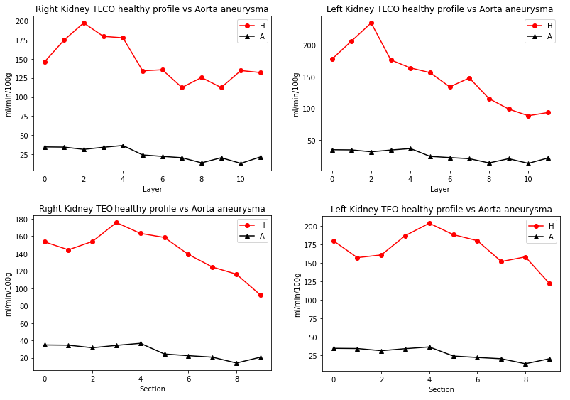
Fig. 4 Healthy volunteers profile vs Aorta aneurysm patient in (a) The TLCO right kidney, (b) The TLCO left kidney, (c) The TEO method in right kidney RBF, (d) The TEO method in left kidney RBF .
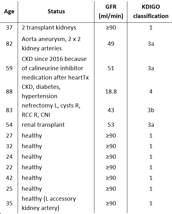
Table 1. Summary of the participants.