Synopsis

Keywords: Data Processing, Diffusion/other diffusion imaging techniques

Q-space trajectory imaging (QTI) is a diffusion MRI framework which access features of the microstructure through the statistical moments of the diffusion tensor distribution. To overcome unreliable estimates obtained with standard fitting methods, a constrained estimation framework named QTI+ was recently proposed. Constrained optimization however typically requires sophisticated fitting routines which introduce a heavy computational burden. In this work we thus explore the possibility of speeding up the QTI parameter estimation, while retaining strict positivity constraints, using artificial intelligence. Results are shown on synthetic datasets as well as for healthy subjects and data from brain tumor patients.

Introduction

Q-space trajectory imaging (QTI)¹ is a diffusion MRI (dMRI) framework combining tensor-encoded diffusion measurements and a diffusion tensor distribution (DTD)² model for the tissue microstructure. The MR signal is represented via cumulant expansion as:
$$ln(S)\,\approx\,ln(S_0)\,-\mathbf{B}:\mathbf{\hat{D}}\,+\frac{1}{2}\,\mathbb{B}:\mathbb{C},$$ where $$$S$$$ is the acquired signal, $$$S_0$$$ is the signal for null diffusion gradients, $$$\mathbf{\hat{D}}$$$ and $$$\mathbb{C}$$$ are, respectively, the second order mean and fourth order covariance tensors of the DTD, and $$$\mathbf{B}$$$ are the measurement tensors. A constrained estimation framework, called QTI+, which imposes relevant positivity conditions on the estimated QTI quantities, was recently introduced by Herberthson et al.³ . Estimates obtained with this framework were shown to both increase the method’s robustness with respect to noise, and lower the requirement on the number of measurements to be collected for the fitting^3,4. However, constrained estimation typically leads to lengthier computations. As previously done by other researchers in the dMRI community^5,6,7,8, in this work we harness the computational efficiency of neural networks to speed up the estimation of QTI parameters while enforcing strict positivity conditions considered in QTI+. We show that QTI metrics produced by the network are comparable to those obtained with QTI+, providing overall smoother maps via shorter computation times.

Methods

$$$\textbf{Positivity}\,\textbf{conditions}$$$
The positivity conditions considered in QTI+ were named d), c), and m) according to which tensor they are enforced upon ($$$\mathbf{\hat{D}},\mathbb{C}\,,$$$ and $$$\,\mathbb{M}=\mathbf{\hat{D}}\otimes\mathbf{\hat{D}}\,+\,\mathbb{C}$$$, respectively). These conditions can be enforced in several steps involving Semidefinite Programming (SDP) and non-linear least squares (NLLS) routines. In this work we consider QTI+ results obtained with the NLLS(dc) routine, which enforces conditions d) and c) using NLLS with initial guess provided by an SDP routine.

$$$\textbf{Neural}\,\textbf{Network}\,\textbf{implementation}$$$
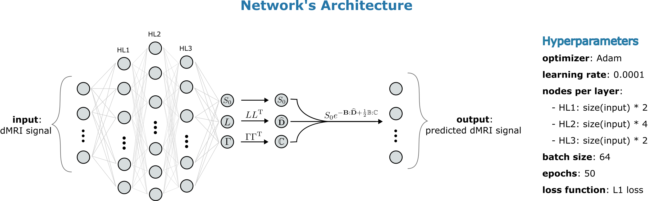
A neural network was implemented using Keras⁹ in TensorFlow¹⁰ in an encoder/decoder architecture. The encoder is a MultiLayer Perceptron (MLP) whose final output is 28 numbers interpreted as being $$$S_0\,,L\,$$$and$$$\,\Gamma$$$, where $$$L$$$ and $$$\Gamma$$$ are lower triangular matrices representing the Cholesky Factorization of $$$\mathbf{\hat{D}}$$$ and $$$\mathbb{C}$$$. The $$$\mathbf{\hat{D}}\,$$$and$$$\,\mathbb{C}$$$ tensors are then obtained as $$$\mathbf{\hat{D}}\,=\,LL^\text{T}\,$$$and$$$\,\mathbb{C}\,=\,\Gamma\Gamma^\text{T}$$$, thus ensuring the satisfaction of conditions d) and c) from QTI+. The decoder then reconstructs the predicted dMRI signal from $$$S_0,\,\mathbf{\hat{D}}$$$, and $$$\mathbb{C}$$$. The network’s architecture, hereafter referred to as ML(dc), and the hyperparameters are displayed in Figure(1). Note that such network is meant to be trained directly on the data of interest, and as such its performance is not affected by possible biases present in the training data. However, it is still possible to train the network on either synthetic or real data, and subsequently deploy it on unseen data to gain additional computational speed.

$$$\textbf{Simulations}\,\textbf{on}\,\textbf{realistic}\,\textbf{brain}\,\textbf{data}$$$
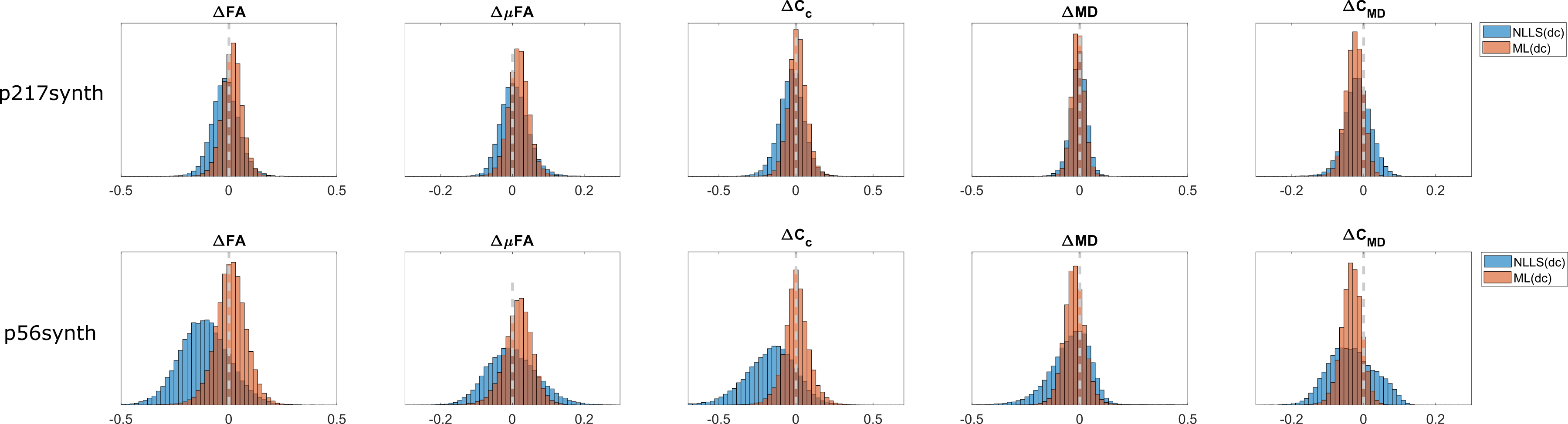
Two realistic healthy brain datasets were generated by computing the QTI signal from parameters obtained by employing QTI+ on a publicly available datasets¹¹ and its subsampled versions. Hereafter these are referred to as p217 and p56 according to the number of diffusion measurements included in the respective sets. Noise from the Rician distribution was added to the synthetic data, hereafter referred to as p217synth and p56synth, to obtain a Signal-to-Noise ratio of 25. The NLLS(dc) and ML(dc) routines’ performances were assessed by computing the difference between the ground truth QTI maps and those obtained with the two method.

$$$\textbf{Clinical}\,\textbf{and}\,\textbf{experimental}\,\textbf{data}$$$
Data from two patients referred for tumor surgery were included in the study after written informed consent (Ethics approval: EPM$$$\,2020-01404$$$). Two protocols were used for the acquisition of the dMRI data: one tumor dataset consisted of 104 diffusion volumes with voxel size $$$2.4\times2.4\times4.8\,\,mm^3$$$, while the other dataset consisted of 70 diffusion volumes with voxel size $$$2.2\times2.2\times2.4\,\,mm^3$$$. Data from a healthy volunteer were also collected with both protocols (Ethics approval:$$$\,2018/143-32$$$). All datasets were preprocessed for motion, eddy currents, and EPI-distortions using tools from FSL¹².

Results

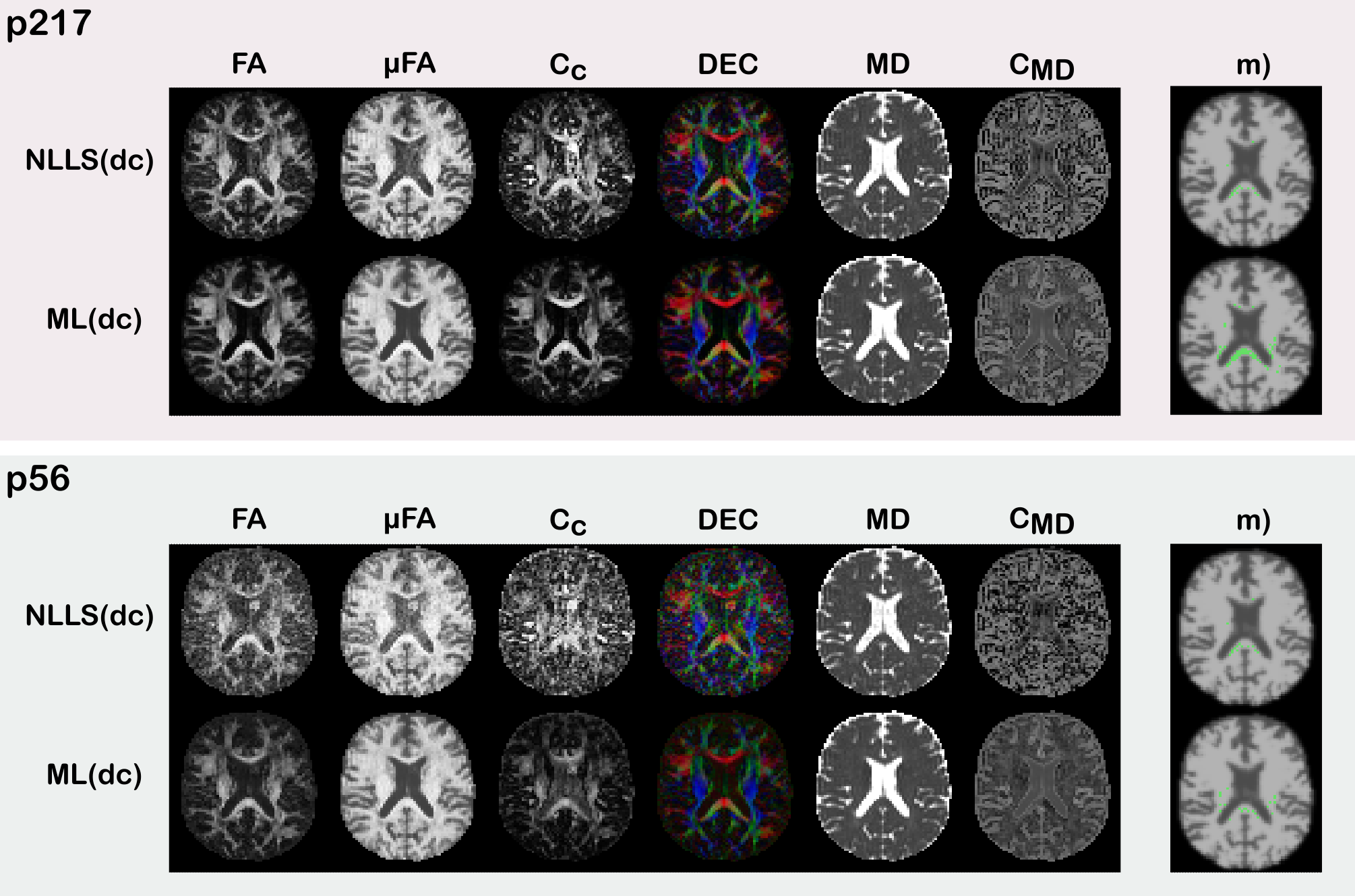
The results in Figure(2) show that ML(dc) produces estimates of similar quality to those of NLLS(dc) in terms of derived QTI-metrics for p217synth, while being markedly better on p56synth. The results also show that ML(dc) exhibits a bias towards reducing anisotropy (quantified by Fractional Anisotropy$$$\,(\textrm{FA})$$$, Microscopic Fractional Anisotropy$$$\,(\mu\textrm{FA})$$$, and Orientational Coherence ($$$\textrm{C}_\text{c}$$$) and increasing Mean Diffusivity ($$$\textrm{MD}$$$) and Size Variance ($$$\textrm{C}_\text{MD}$$$). This is probably due to an intrinsic denoising process occurring during network training.

The maps in Figure(3) show superior quality for the estimates produced with ML(dc), especially when fewer dMRI volumes are available.

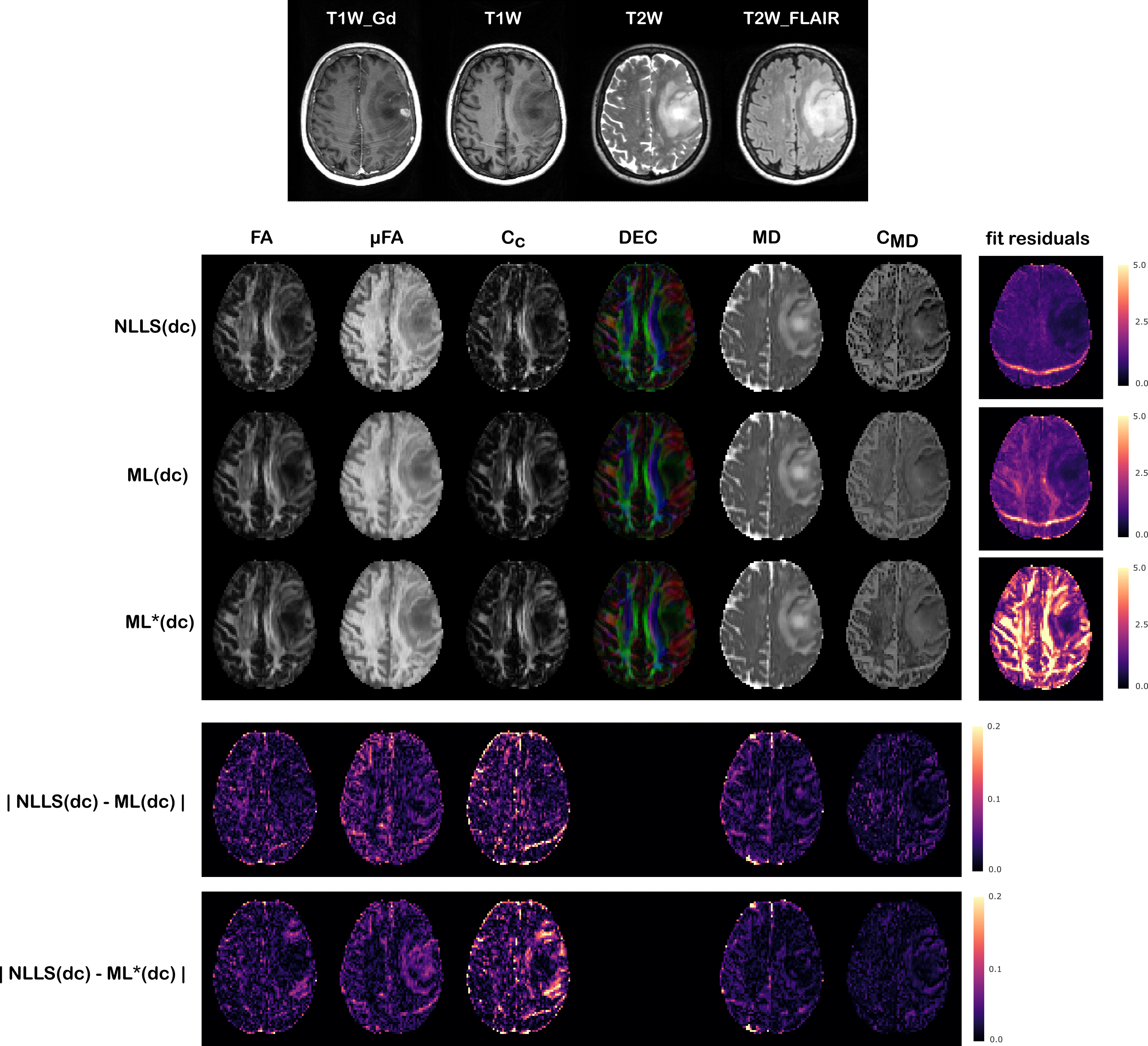
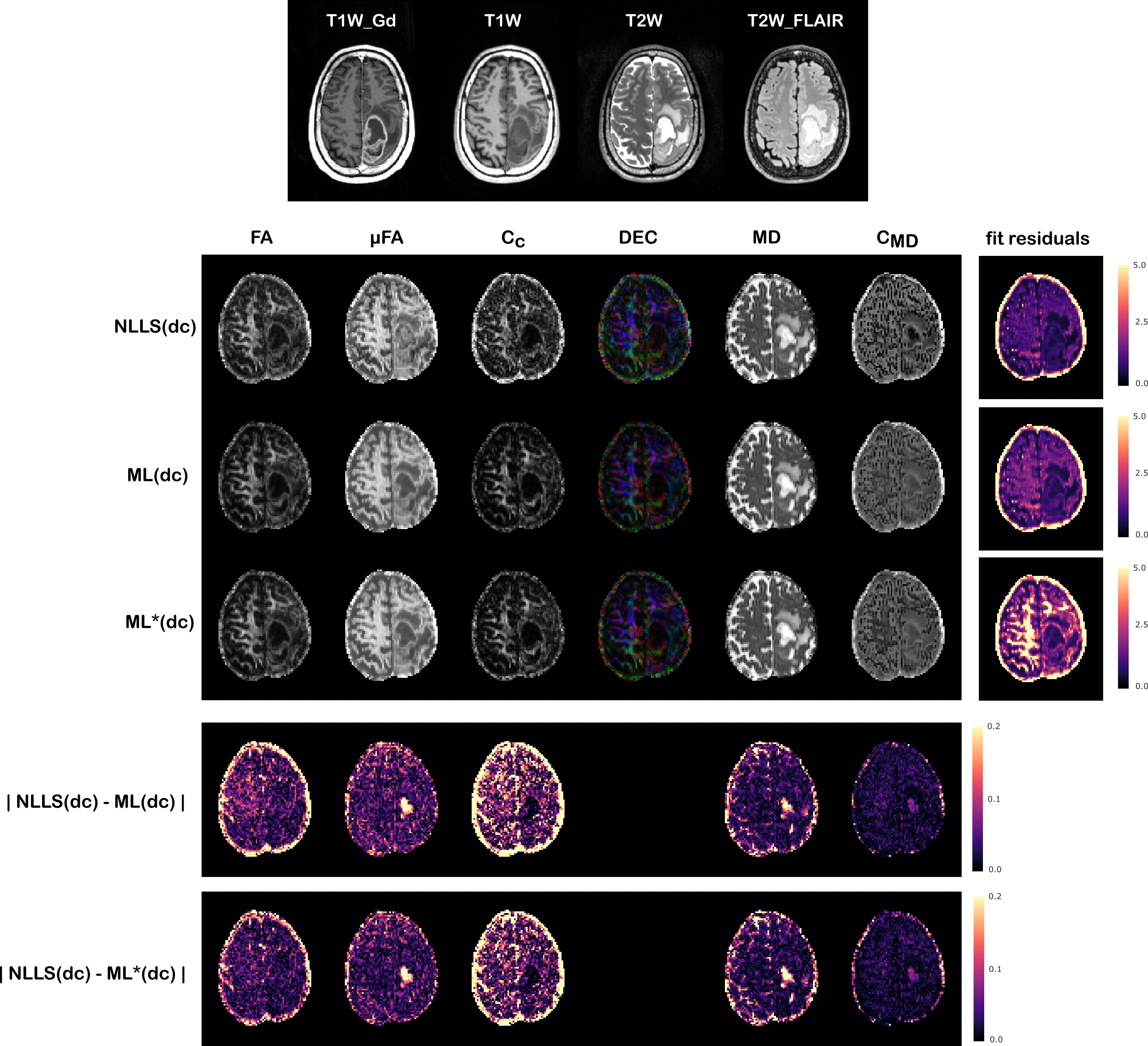
Figures(4)$$$\,$$$and$$$\,$$$(5) show the results obtained on the two tumor datasets, for both a network trained directly on the tumor data (ML(dc)), and a network trained on the healthy volunteer data and then deployed on the patients’ data (ML*(dc)). Despite higher fitting residuals, the ML*(dc) net produces similar QTI maps to ML(dc). Compared to NLLS(dc), both ML strategies produce visibly smoother results which seems to better highlight certain details about the tumor’s microenvironments, but at the same time could be removing precious details. Computations took on average 0.4 seconds for ML*(dc), 3 minutes for ML(dc), and 40 minutes for NLLS(dc).

Discussion & Conclusion

Similarly to previous dMRI studies^5,6,7,8, this work also suggests neural networks as a valuable alternative to standard fitting routines, especially when computational time is a concern. In conclusion, we presented a neural network architecture in which model constraints are enforced. This approach could be applied to other dMRI methods for which positivity constraints are available¹³.

Acknowledgements

The authors thank the staff at the Department of Neurosurgery at Linköping University Hospital and Elisabeth Klint, MSc, and Karin Wårdell, PhD, from the Department of Biomedical Engineering, Linköping University, for data collection. This project was financially supported by the Swedish Foundation for Strategic Research (RMX18-0056), Linköping University Center for Industrial Information Technology (CENIIT), Sweden's Innovation Agency (VINNOVA) ASSIST, and Analytic Imaging Diagnostic Arena (AIDA).