3717
A noise robust image reconstruction deep neural network with cycle interpolation
Jeewon Kim1, Wonil Lee1, Beomgu Kang1, Seohee So2, and HyunWook Park1
1Korea Advanced Institute of Science and Technology (KAIST), Daejeon, Korea, Republic of, 2Korea Institute of Science and Technology, Seoul, Korea, Republic of
1Korea Advanced Institute of Science and Technology (KAIST), Daejeon, Korea, Republic of, 2Korea Institute of Science and Technology, Seoul, Korea, Republic of
Synopsis
Keywords: Machine Learning/Artificial Intelligence, Parallel Imaging
We propose a new Parallel Imaging scheme using a deep neural network which performs well with fewer ACS line in noisy environments. The proposed scheme includes ACS loss which is used in RAKI and cycle interpolation loss that we newly propose in our work. RAKI generalized GRAPPA in noisy environments by applying non-linear k-space interpolation with a deep neural network. However, it requires additional ACS lines to output satisfactory performance. Here, we suggest a new scheme to overcome the reconstruction performance in a noisy environment with fewer ACS lines.Introduction
Magnetic resonance imaging (MRI) provides a variety of useful clinical information widely used in clinical diagnosis. However, MRI requires a long scan time, which results in high cost. Therefore, accelerating the scan has been a constant topic of research. To reduce the burden of acquiring signals, Parallel Imaging (PI) has been studied. GRAPPA is a traditional algorithm that reconstructs missing k-space data by using shift-invariant convolutional kernels which can be described by a linear convolution across all channel data in k-space1. With the development of deep learning, RAKI introduced a convolutional kernel with a neural network where non-linear activation function was applied2. Both methods estimate kernels by using an autocalibration signal (ACS). However, acquiring more ACS lines requires a longer scan time. Therefore, obtaining smaller number of ACS lines plays a crucial role in reducing the scan time. As GRAPPA is weak against noisy environments and RAKI requires more ACS lines to provide better performance, we propose a cycle interpolator network to overcome both problems.Method
Cycle Interpolator: Subsampled zero-filled k-space is the input of $$$Net_i$$$, where the real part of the k-space is concatenated with the imaginary part of the k-space along the channel direction ($$$1\leq i \leq 2n_c$$$, $$$n_c$$$= number of coils). Each $$$Net_i$$$ estimates missing lines of each coil data where the parameters of the $$$Net_i$$$ functions as the GRAPPA kernel. Estimated missing lines of each coil are then used to re-estimate the subsampled k-space lines. We obtain a loss between the subsampled k-space and the re-estimated subsampled k-space which is named cycle interpolator loss ($$$\mathcal{L_{Cycle}}$$$). Fig.1A describes the cycle interpolator network with a reduction factor (R) of two. The ACS loss ($$$\mathcal{L_{ACS}}$$$) is the loss between ACS lines and the estimated ACS lines by the (Fig.1B). The total loss is the sum of the cycle interpolator loss and ACS loss ($$$\mathcal{L_{Tot}}=\mathcal{L_{Cycle}}+\mathcal{L_{ACS}}$$$).Neti: The proposed method used the same neural network architecture used in RAKI implemented with pyTorch. Three convolution layers with ReLU are used and the details of each layer are described in Fig.1C. The convolution utilizes a kernel size of PE (phase encoding) x RO (readout) with a dilation rate of R in the PE direction. The numbers 32, 8, R-1 in Fig.1C represent the channel size.
In-vivo Experiments: MRI experiments on healthy volunteer were performed on a 3T MRI scanner (Magnetom Verio, Siemens Healthcare, Germany) with a 12-channel head coil. The experiments were performed with the spin-echo based T1w imaging sequence having the following imaging parameters: TR/TE = 558/9.8 ms; FOV = 220x220 mm2; matrix size = 384x384. MR signals were fully sampled in the k-domain without acceleration. Each k-space data was retrospectively subsampled with a reduction factor (R) of 2-4. 23 ACS lines (6%) were used.
Results
Using only 23 ACS lines (6%) for the T1-dataset at R = 2-4, the cycle interpolator network outperforms RAKI by suppressing aliasing artefacts. Also, the network preserves structures more accurately than the other methods even in noisy environments. To emphasize the noisy environments, imaging was performed by selecting a thinner slice thickness. While the cycle interpolator network performs well in all cases, its performance compared to other methods is best at R=4 as shown in Figs.2-4. RAKI results in aliasing artefacts and blurred brain structures, while GRAPPA results in noisy images that blur the structure. In the case with substantial noise in the thinner slices (1mm), RAKI results in noisy reconstructions, while GRAPPA results in a reconstruction that has an unrecognizable CSF region in R=4. The enhanced performance is also indicated by the quantitative image quality metrics of NMSE, PSNR, and SSIM (Figs.2-4).Discussion
Cycle interpolator network outperforms RAKI and GRAPPA in 2D imaging with less ACS lines (6%) and noisy environments. By extending upon GRAPPA’s concept that missing k-space lines can be estimated with space invariant kernels, the cycle interpolator network is able to re-estimate the acquired lines from the estimated missing lines, which in turn increases the accuracy of the reconstruction. With the help of neural networks, the cycle interpolator network provides better performance in noisy environments compare to GRAPPA. Also, by adding a cycle interpolator loss to the original ACS loss used in RAKI, the cycle interpolator network reconstructs images better than RAKI with less ACS lines. Unlike the other deep learning methods which require a large training dataset, the cycle interpolator network is a database-free deep learning like RAKI. As it is a scan-specific reconstruction, it prevents the reconstruction of hallucinations that have occurred in other networks trained with large dataset3.Conclusion
The number of ACS is essential in RAKI, and the noisy environment hampers the performance of GRAPPA as reduction factor (R) increases. With less ACS lines and noisy environments, the cycle interpolator network provides improved reconstruction quality compared to RAKI and GRAPPA while preserving the structure information of the brain with improved noise resilience.Acknowledgements
This work was supported by the Korea Medical Device Development Fund grant funded by the Korea government (the Ministry of Science and ICT, the Ministry of Trade, Industry and Energy, the Ministry of Health & Welfare, the Ministry of Food and Drug Safety) (Project Number: 1711138003, KMDF-RnD KMDF_PR_20200901_0041-2021-02).References
[1] Griswold MA, et al. Generalized autocalibrating partially parallel acquisitions (GRAPPA). Magnetic Resonance in Medicine 2002;47(6):1202–1210.
[2] Akçakaya M, et al. Scan-specific robust artificial-neural-networks for k-space interpolation (RAKI) reconstruction: Database-free deep learning for fast imaging. Magnetic Resonance in Medicine 2019;81(1):439–453.
[3] Muckley, Matthew J., et al. "Results of the 2020 fastmri challenge for machine learning mr image reconstruction." IEEE transactions on medical imaging 40.9 (2021): 2306-2317.
Figures
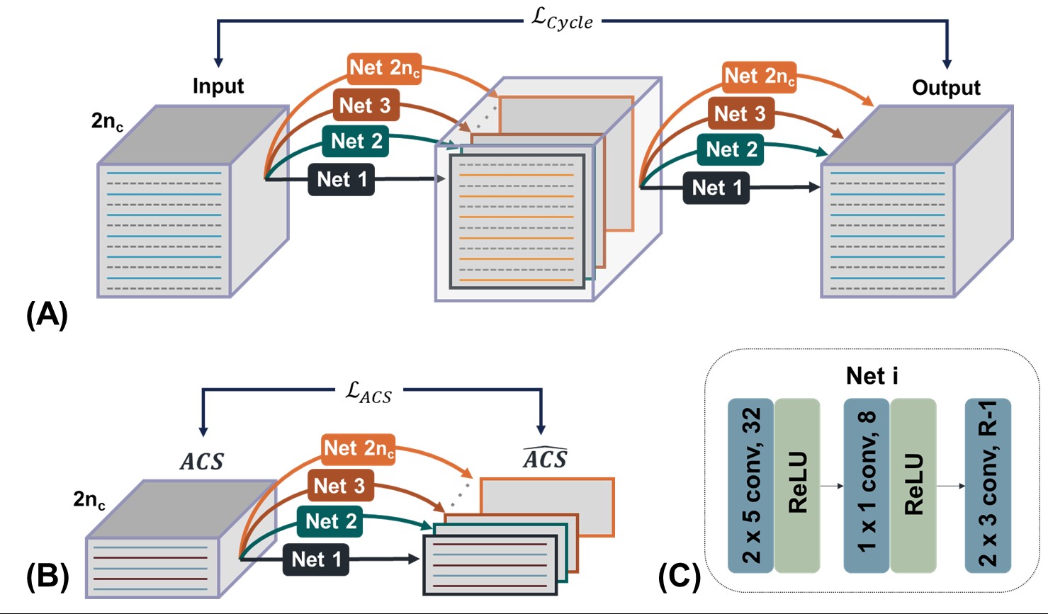
Figure 1. Schematic diagram of the proposed method.
(A) By passing each Neti twice, subsampled
zero-filled k-space input data is re-estimated. The loss between the input and the re-estimated subsampled k-space ($$$\mathcal{L_{Cycle}}$$$) is used to optimize each Neti.
(B) The ACS lines are estimated by each Neti.
The loss between ACS lines and the
estimated ACS lines ($$$\mathcal{L_{Cycle}}$$$) is used to optimize each Neti. (C) Neti: The 3-layer CNN with ReLU is
used. The kernel size of 2x5, 1x1, and 2x3 are used, respectively, with a
dilation rate of R in PE direction.
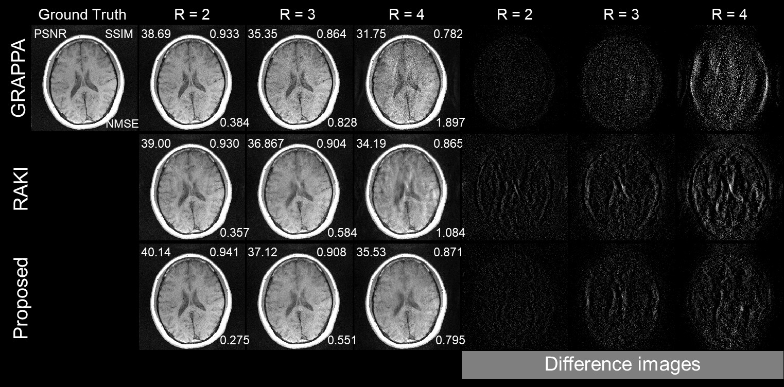
Figure
2.
GRAPPA (top), RAKI (middle), and proposed method (bottom) in comparison for reconstruction of T1w dataset
acquired with 5mm thickness at R=2-4 using 23 ACS lines (6%).

Figure
3.
GRAPPA (top), RAKI (middle), and proposed
method (bottom) in comparison for reconstruction of T1w dataset acquired with
3mm thickness at R=2-4 using 23 ACS lines (6%).
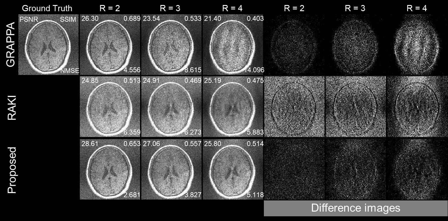
Figure
4.
GRAPPA (top), RAKI (middle), and
proposed method (bottom) in comparison for reconstruction of T1w dataset
acquired with 1mm thickness at R=2-4 using 23 ACS lines (6%).
DOI: https://doi.org/10.58530/2023/3717